Image Classification Explained [+V7 Tutorial]

Training

So, we got our data and our model, but how do we train it to successfully classify images?

Well, first of all, you need to know that there are two main categories of learning.

Supervised Learning

When we provide our model with training errors signals, e.g. you classify this image as a cat but it was a dog, we perform supervised learning. This is the most common scenario in which we have labeled datasets with image and class pairs.

Neural Networks are trained by minimizing a function, called loss, using gradient descend.

For single-label classification, we rely on the, defined as follows:

Don't be scared by the notation, m is the number of samples, y_i is the label, hat y_i is the prediction and ln is the natural logarithm.

Softmax

The model outputs a vector with a length equal to a number of classes, they are the classes' scores. Since they can be anything, we apply a special function called Softmax.

It makes these numbers sum up to one, so each individual item is bounded between 0 and 1. The more close to one the model thinks that class is the correct one.

The Softmax is defined as follows.

So we take the exponential of the output and we divide by the sum of the exponential of all the outputs. Let's take an example, imagine we have two classes and our output is:

Clearly, the value for class 2, hat y_2, is the biggest one, but we really want them to be between 0 and 1 (you'll see it later). So let's apply the function, first let's find the denominator.

Then we take the exponential of each output and we divide by it.

The number sums up to one and they capture the correct score the model assigned previously. You may are wondering why we don't just normalize the output.

Here's the answer—

If we normalize the previous values we obtain [0.28, 0.71], while if with Softmax [0.05, 0.95]. Softmax pushes the values more away than vanilla normalization, effectively almost taking the maximum value, this is from where the name Softmax comes from.

Cross Entropy

Let's take an example if our target is $0$ but our model output $0.9$, so very close to $1$, the loss value would be.

Remember, in this case, the model outputs a vector with a length equal to a number of classes, they are the class's score. These numbers sum up to one, so each individual item is bounded between 0 and 1.

The more to close to one the model thinks that class is the correct one.

If you know about regression you may think that we can apply Mean Square Error and call if a day.

MSE doesn't penalize the model as much as BCE does. If we compute the gradient with respect to hat y_i.

While with MSE:

The gradient from BCE is 5 times more, thus the model will be penalized more.

Multi-Labels Classification

For multi-labels classification we want our outputs to be independent of each other since multi classes can exist at the same time. For example, if we have two classes at the same time our output could be [20, 21], we cannot apply Softmax since it will give more importance to one specific value, the biggest one.

In this case, we apply the Sigmoid function before BCE that maps between [-1,1], it is defined as follows.

This will make sure that each individual value in our model outputs is bounded by the same range.

Unsupervised Learning

Here we don't have annotations, just a big collection of raw images and we let our model figure out what they are during training.

There are different approaches to solving this task—let's go through each one of them.

Contrastive learning

In contrastive learning, we take an input image, x, sample a “positive” image, x_pos, and a “negative” image, x_pos, in some way and try to train a scoring model such that score(x, x_pos) > score(x, x_neg)

A sample with positive and negative images

We draw these samples randomly by enforcing that each time we have a different positive and negative example.

If we have labels, the negative sample must be from a different class, while the positive one is from the same one. When there are missing labels, one easy way to get the sample is to sample two parts of the same image for the positive and one part of another random image for the negative.

Sample of the same image negative and positive

Given a vector representation of an image, we try to push the two positive as close as possible and the negative them far away. One way is to learn a similarity metric, D.

D is the distance between these representations.

If positive, we want our loss L to push them close.

So we want x and x_pos to have a big dot product. On the other hand, if we have a negative sample we do the opposite.

The epsilon acts like a margin value.

Depending on how we decide to sample our example, we can have a pairwise loss, so with (x, x_pos) and (x, x_neg) or a triplet loss with (x, x_pos, x_neg) all together.

With Tripet losses, we first compute the score between x,_pos and x and x_neg, and then we use them in the loss.

Our variable m acts like a margin.

Another very common loss is InfoNCE in which here we can have multiple negative examples.

InfoNCE is the log-likelihood to predict the correct example from a given set of examples based on the score of the model.

The score function, s, is usually the inner product. The higher the more similar they are and vice versa.

One very successful method that uses contrastive learning is SimCLR in which you have a network f, usually a ResNet-50, and a linear projection, g.

The way it works is simple—

We sample a minibatch from the dataset and for each data point, x, we apply data augmentation and pass them through the network, f, and the linear projection obtained two representations. This effectively creates two positive pairs since we augmented the same images, then we apply a contrastive loss on all the augmented data points in the batch keeping track of the positive pairs.

Generative Models

Another idea is to tackle the unsupervised problem by using generative networks.

The idea is to give the networks reconstruction images tasks.

For example, we can crop some part of the image and train the network to fill in the gap.

Generative model

This task requires the network to develop context-aware skills to reconstruct the missing input. Unfortunately, there are some limitations to this approach.

For example, there are way too many pixels details that the network has to learn that are not essentials, like the color.

Pro tip: To learn more, check out this Introduction to Autoencoders.

We can overcome these issues by using some ideas from contrastive learning, like applying an augmentation to create a pair of positive examples and training the network to reconstruct the permuted example.

However, there are some caveats here as well—

To make this work we also need a lot of negative examples, which is not ideal.

Teacher student models

One of the most efficient methodologies is the teacher-student approach.

The teacher and the student are two networks, usually the same. An input image, x, is first augmented in two different ways and then each of the new augmented images is passed to the teacher and student respectively.

They generate two features vector that we score with a reconstruction loss, like Mean Square Error or Cosine Similarity. Since they come from the same image, they are a positive pair and we want the result features from both models to be as similar as possible.

We don't need negative examples.

One approach that we want to highlight here is BYOL.

In BYOL, at each training step, after creating two augmented images from a data point and computing their score in the features space, the parameters of the student are updated using gradient descent while the teacher's ones are updated with the exponential moving average of the student's weights.

Even though it is a very straightforward procedure, it is highly effective.

Image Classification Metrics

Image Classification models have to be evaluated to determine how well they perform in comparison to other models.

Here are some well-known metrics used in Image Classification.

Precision

Precision is a metric that is defined for each class. Precision in a class tells us what proportion of data predicted by the ML model to belong to the class was actually part of the class in the validation data.

A simple formula can demonstrate this:

Where:

• TP represents True Positives: The number of samples that were predicted to belong to a class and correctly belong to the class.

• FP represents False Positives: The number of samples that were predicted to belong to a class while they do not belong to the class at all.

Recall

Recall similar to precision is defined for each class.

Recall tells us what proportion of the data from the validation set belonging to the class was identified correctly (as belonging to the class). 

Recall can be represented as:

Where:

• FN represents False Negatives: The number of samples that the model predicted as not belonging to a class while they actually belong to that particular class.

F1 Score

F1 Score helps us achieve a balance between precision and recall to get an average idea of how the model performs.

F1 score as a metric is calculated as follows.

Precision and Recall scores largely depend on the problem the classification model is trying to address.

Recall is a critical metric, particularly in problems referring to the medical image analysis, like detection of pneumonia from chest X-rays, where false negatives cannot be present to prevent diagnosing a patient as healthy when they actually have the disease.

Precision is needed where the false positives have to be avoided, like email spam detection. If an important email is classified as spam, then a user would face significant issues.

Bonus 1: Video classification explained

Significantly differing from Image Classification, which only uses Image Processing algorithms and Convolutional Neural Networks to make a classification, Video Classification tasks make use of both image and temporal (relating to time) data.

Video Classification algorithms utilize the relation between the various frames in a continuous video to perform better than standard Image Classification algorithms on these tasks.

Neural Networks better suited to time series data like LSTMs (Long Short Term Memory) and RNNs (Recurrent Neural Networks) are used in conjunction with CNNs to perform video classification tasks to exploit the temporal relations between frames that simple CNN based methods would miss out on.

General Video classification datasets include sports datasets and datasets obtained from Youtube.

Bonus 2: 3D Classification explained

3D data classification is very similar to 2D image classification, with the primary difference being in the structure of the CNN and the nature of the movement of the sliding kernel.

Kernels in 3D data classification are also 3D and move along all three axes as compared to two axes linear motion in 2D CNNs.

CNNs are adept in capturing spatial data and hence adapt easily when the data is spaced out over three axes as compared to two.

Popular 3D classification datasets are found in the medical domain, with brain data obtained from MRI scans and structural data of macromolecules obtained from Cryo-Electron Microscopy.

How to train an image classifier on V7?

Finally, let us walk you through the process of training image classification models on V7. No matter your experience level, V7 makes it extremely easy to build reliable image classifiers within minutes.

To begin, you need to sign up for a 14-day free trial to get access to our tool. And once you are in, here's what comes next.

1. Upload the data

To start building an image classifier on V7, you need to upload image data that you want to work with. Go to the dataset tab on the left-hand side of the screen and click “New Dataset”.

V7 also allows you to upload your data via API and CLI SDK.

Pro tip: For more information, make sure to check out V7 Darwin Documentation.

2. Create new annotation classes (tags)

You can do it both ways—either from the image level or going to the "Classes tab to create your classes in bulk.

New annotation class creation on V7

Apart from choosing your annotation type—in this case a tag, you can also add subannotations, such as Attributes or Text.

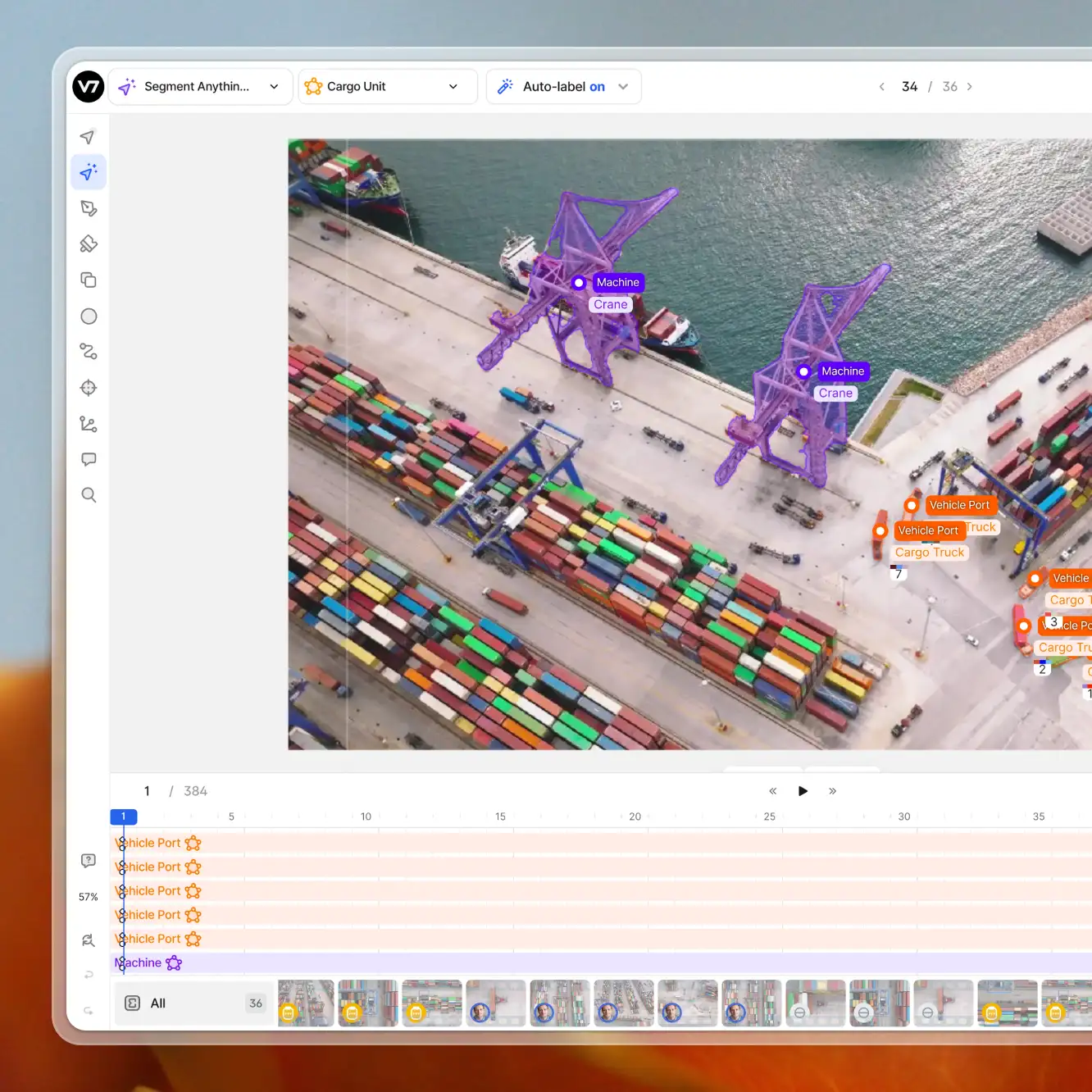
3. Annotate your data (image tagging)

Once you've created your classes and organized your dataset, you can start labeling your data by adding tags to your images. As mentioned above, you can either add your tags to each image individually or tag them in bulk from the dataset level.

Tagging a colibri on V7

4. Train your Image Classification model

Once you've annotated enough instances, you are ready to train your first image classifier using V7!

Simply head over to the "Neural Networks" tab, add new model, choose "Image Classification", pick your dataset and start training.

Training Image Classification model on V7

And... don'rt forget that V7 also allows you to train object detection, instance segmentation and OCR models ;-)

Now, go ahead, and start building your AImodels! We are excited to see your computer vision project ideas.

Image classification in a nutshell: Key takeaways

Finally, let's recap everything you've learned today about image classification:

• Image classification is a subdomain of computer vision dealing with categorizing and labeling groups of pixels or vectors within an image using a collection of predefined tags or categories that an algorithm has been trained on.

• We can distinguish between supervised and unsupervised classification.

• In supervised classification, the classification algorithm is trained on a set of images along with their corresponding labels.

• In unsupervised classification, the algorithm uses only raw data for training.

• To build reliable image classifiers you need enough diverse datasets with accurately labeled data.

• Image classification with CNN works by sliding a kernel or a filter across the input image to capture relevant details in the form of features.

• The most important image classification metrics include Precision, Recall, and F1 Score.

Read more:

Annotating With Bounding Boxes: Quality Best Practices

YOLO: Real-Time Object Detection Explained

The Beginner’s Guide to Semantic Segmentation

A Comprehensive Guide to Human Pose Estimation

‍