Autoencoders in Deep Learning: Tutorial & Use Cases [2023]

Ready to streamline AI product deployment right away? Check out:

What is an autoencoder?

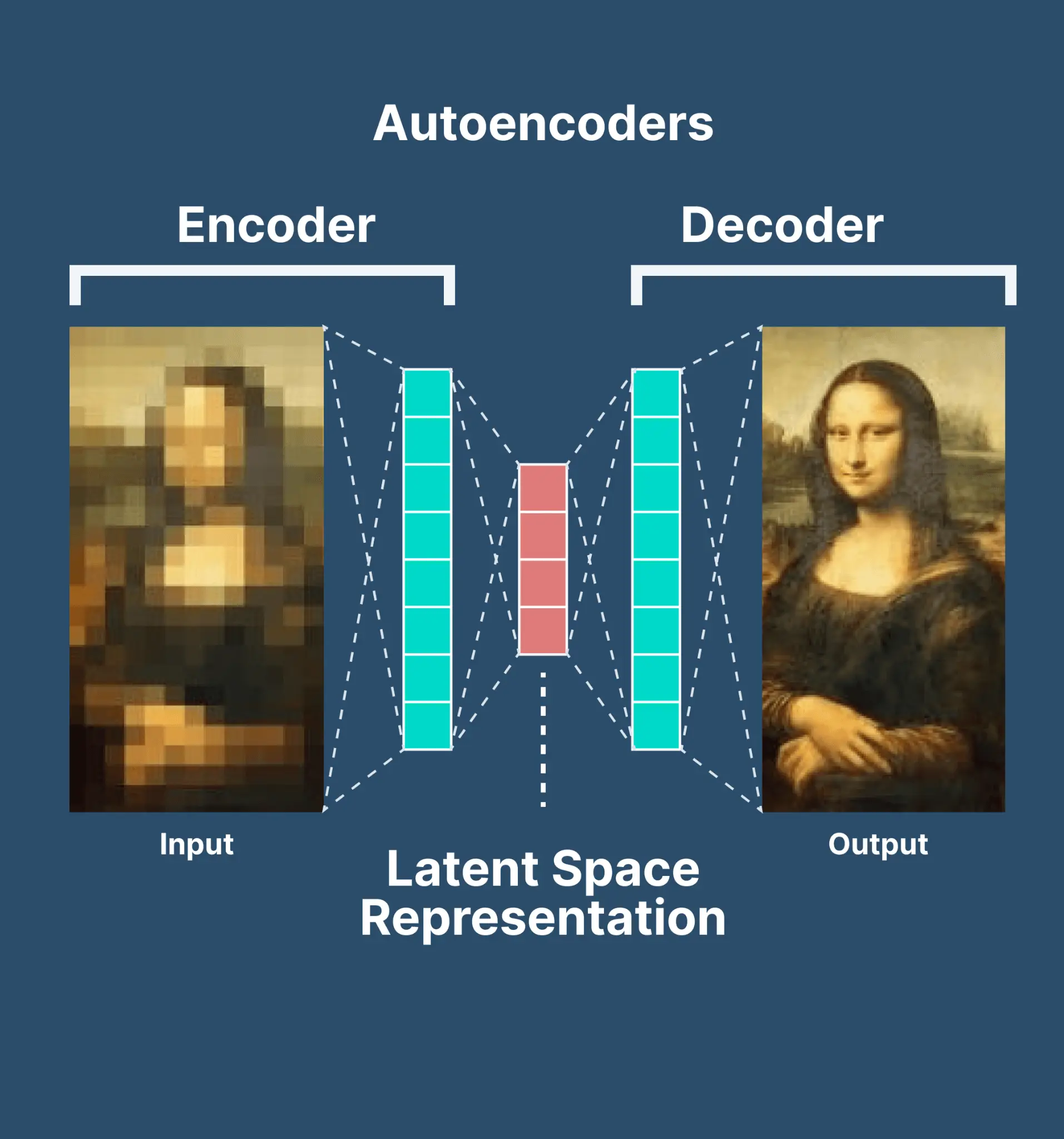
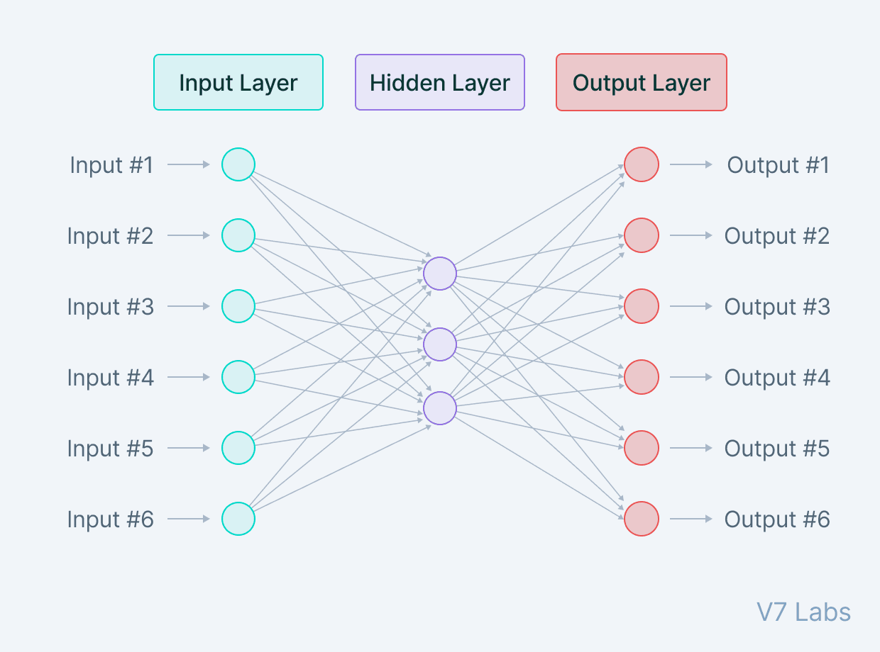
An autoencoder is a type of artificial neural network used to learn data encodings in an unsupervised manner.

The aim of an autoencoder is to learn a lower-dimensional representation (encoding) for a higher-dimensional data, typically for dimensionality reduction, by training the network to capture the most important parts of the input image.

💡 Pro tip: Check out Supervised vs. Unsupervised Learning

The architecture of autoencoders

Let’s start with a quick overview of autoencoders’ architecture.

Autoencoders consist of 3 parts:

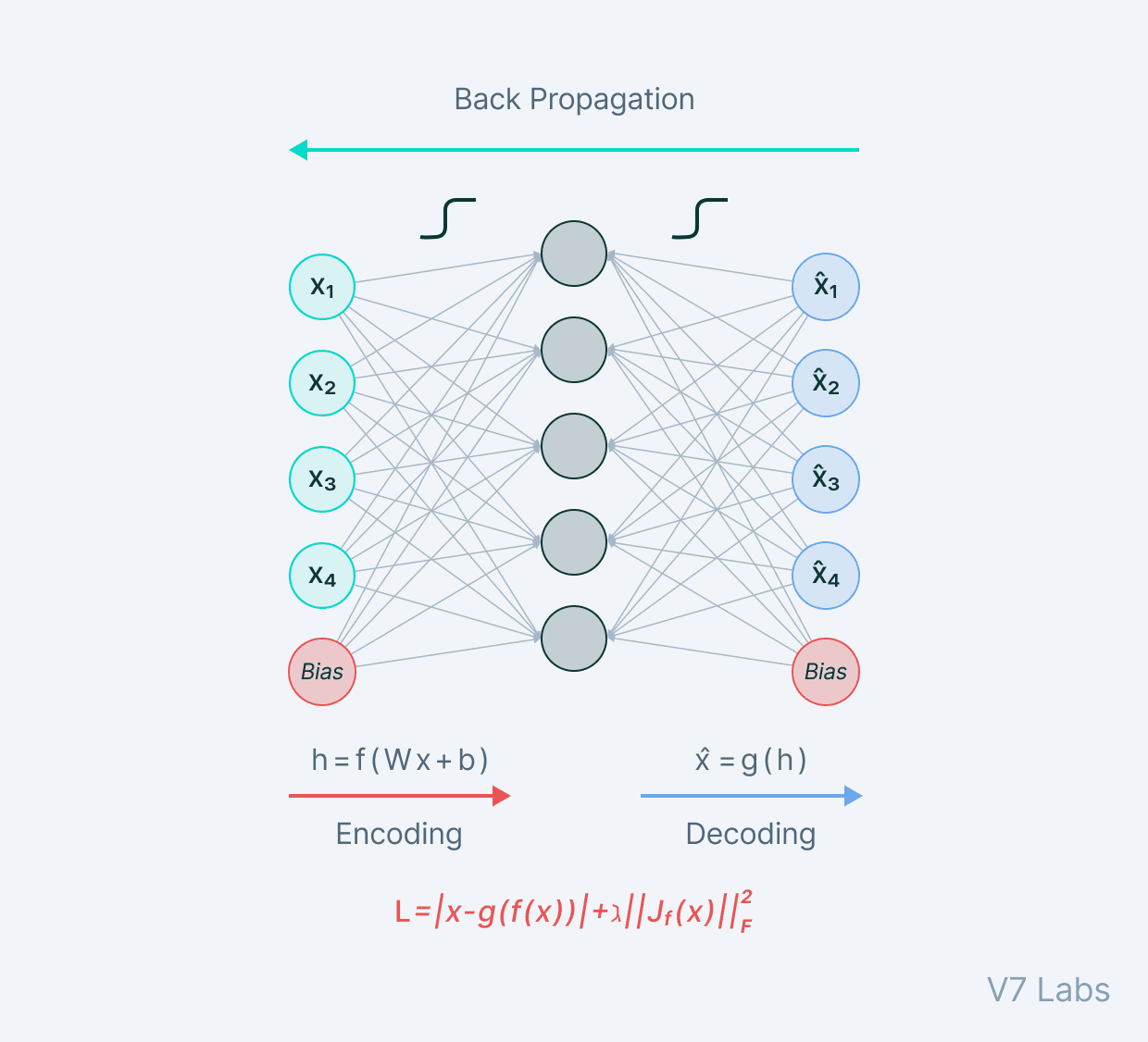
1. Encoder: A module that compresses the train-validate-test set input data into an encoded representation that is typically several orders of magnitude smaller than the input data.

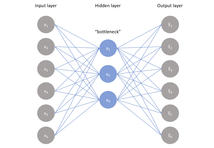
2. Bottleneck: A module that contains the compressed knowledge representations and is therefore the most important part of the network.

3. Decoder: A module that helps the network“decompress” the knowledge representations and reconstructs the data back from its encoded form. The output is then compared with a ground truth.

The architecture as a whole looks something like this:

Ready to explore this topic more in-depth?

Let’s break it down.

The relationship between the Encoder, Bottleneck, and Decoder

Encoder

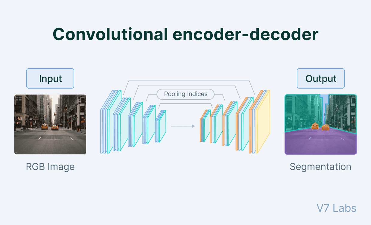
The encoder is a set of convolutional blocks followed by pooling modules that compress the input to the model into a compact section called the bottleneck.

The bottleneck is followed by the decoder that consists of a series of upsampling modules to bring the compressed feature back into the form of an image. In case of simple autoencoders, the output is expected to be the same as the input data with reduced noise.

However, for variational autoencoders it is a completely new image, formed with information the model has been provided as input.

Bottleneck

The most important part of the neural network, and ironically the smallest one, is the bottleneck. The bottleneck exists to restrict the flow of information to the decoder from the encoder, thus,allowing only the most vital information to pass through.

Since the bottleneck is designed in such a way that the maximum information possessed by an image is captured in it, we can say that the bottleneck helps us form a knowledge-representation of the input.

Thus, the encoder-decoder structure helps us extract the most from an image in the form of data and establish useful correlations between various inputs within the network.

A bottleneck as a compressed representation of the input further prevents the neural network from memorising the input and overfitting on the data.

As a rule of thumb, remember this: The smaller the bottleneck, the lower the risk of overfitting.

However—

Very small bottlenecks would restrict the amount of information storable, which increases the chances of important information slipping out through the pooling layers of the encoder.

Decoder

Finally, the decoder is a set of upsampling and convolutional blocks that reconstructs the bottleneck's output.

Since the input to the decoder is a compressed knowledge representation, the decoder serves as a “decompressor” and builds back the image from its latent attributes.

How to train autoencoders?

You need to set 4 hyperparameters before training an autoencoder:

Code size: The code size or the size of the bottleneck is the most important hyperparameter used to tune the autoencoder. The bottleneck size decides how much the data has to be compressed. This can also act as a regularisation term.

Number of layers: Like all neural networks, an important hyperparameter to tune autoencoders is the depth of the encoder and the decoder. While a higher depth increases model complexity, a lower depth is faster to process.

Number of nodes per layer: The number of nodes per layer defines the weights we use per layer. Typically, the number of nodes decreases with each subsequent layer in the autoencoder as the input to each of these layers becomes smaller across the layers.

Reconstruction Loss: The loss function we use to train the autoencoder is highly dependent on the type of input and output we want the autoencoder to adapt to. If we are working with image data, the most popular loss functions for reconstruction are MSE Loss and L1 Loss. In case the inputs and outputs are within the range [0,1], as in MNIST, we can also make use of Binary Cross Entropy as the reconstruction loss.

💡 Pro tip: Looking for quality training data? Check out 65+ Best Free Datasets for Machine Learning to find the right dataset for your needs.

Finally, let’s explore different types of autoencoders that you might encounter.

5 types of autoencoders

The idea of autoencoders for neural networks isn't new.

In fact—

The first applications date to the 1980s. Initially used for dimensionality reduction and feature learning, an autoencoder concept has evolved over the years and is now widely used for learning generative models of data.

Here are five popular autoencoders that we will discuss:

Undercomplete autoencoders
Sparse autoencoders
Contractive autoencoders
Denoising autoencoders
Variational Autoencoders (for generative modelling)

1. Undercomplete autoencoders

An undercomplete autoencoder is one of the simplest types of autoencoders.

The way it works is very straightforward—

Undercomplete autoencoder takes in an image and tries to predict the same image as output, thus reconstructing the image from the compressed bottleneck region.

Undercomplete autoencoders are truly unsupervised as they do not take any form of label, the target being the same as the input.

The primary use of autoencoders like such is the generation of the latent space or the bottleneck, which forms a compressed substitute of the input data and can be easily decompressed back with the help of the network when needed.

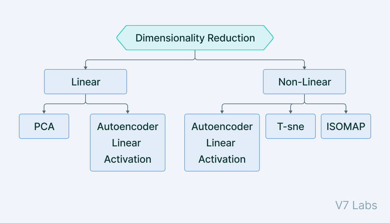
This form of compression in the data can be modeled as a form of dimensionality reduction.

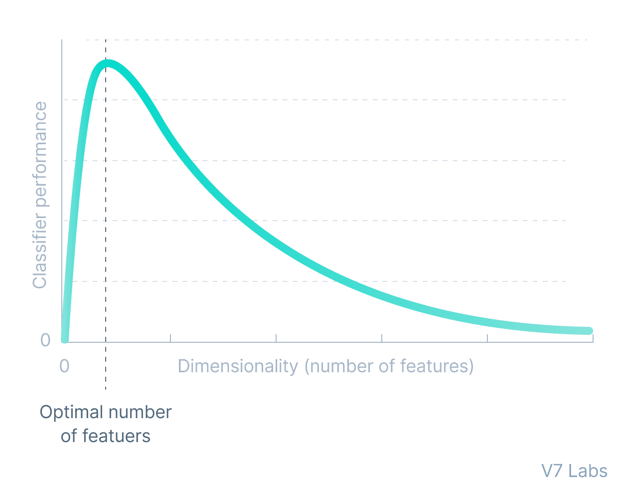
When we think of dimensionality reduction, we tend to think of methods like PCA (Principal Component Analysis) that form a lower-dimensional hyperplane to represent data in a higher-dimensional form without losing information.

However—

PCA can only build linear relationships. As a result, it is put at a disadvantage compared with methods like undercomplete autoencoders that can learn non-linear relationships and, therefore, perform better in dimensionality reduction.

This form of nonlinear dimensionality reduction where the autoencoder learns a non-linear manifold is also termed as manifold learning.

Effectively, if we remove all non-linear activations from an undercomplete autoencoder and use only linear layers, we reduce the undercomplete autoencoder into something that works at an equal footing with PCA.

The loss function used to train an undercomplete autoencoder is called reconstruction loss, as it is a check of how well the image has been reconstructed from the input data.

Although the reconstruction loss can be anything depending on the input and output, we will use an L1 loss to depict the term (also called the norm loss) represented by:

‍

L = |x - \hat{x}|

‍

Where $\hat{x}$ represents the predicted output and x represents the ground truth.

As the loss function has no explicit regularisation term, the only method to ensure that the model is not memorising the input data is by regulating the size of the bottleneck and the number of hidden layers within this part of the network—the architecture.

2. Sparse autoencoders

Sparse autoencoders are similar to the undercomplete autoencoders in that they use the same image as input and ground truth. However—

The means via which encoding of information is regulated is significantly different.

While undercomplete autoencoders are regulated and fine-tuned by regulating the size of the bottleneck, the sparse autoencoder is regulated by changing the number of nodes at each hidden layer.

Since it is not possible to design a neural network that has a flexible number of nodes at its hidden layers, sparse autoencoders work by penalizing the activation of some neurons in hidden layers.

In other words, the loss function has a term that calculates the number of neurons that have been activated and provides a penalty that is directly proportional to that.

This penalty, called the sparsity function, prevents the neural network from activating more neurons and serves as a regularizer.

While typical regularizers work by creating a penalty on the size of the weights at the nodes, sparsity regularizer works by creating a penalty on the number of nodes activated.

This form of regularization allows the network to have nodes in hidden layers dedicated to find specific features in images during training and treating the regularization problem as a problem separate from the latent space problem.

We can thus set latent space dimensionality at the bottleneck without worrying about regularization.

There are two primary ways in which the sparsity regularizer term can be incorporated into the loss function.

L1 Loss: In here, we add the magnitude of the sparsity regularizer as we do for general regularizers:

‍

L = |x - \hat{x}| + λ \sum_{i} |{a_{i}}^{(h)}|

Where h represents the hidden layer, i represents the image in the minibatch, and a represents the activation.

KL-Divergence: In this case, we consider the activations over a collection of samples at once rather than summing them as in the L1 Loss method. We constrain the average activation of each neuron over this collection.

Considering the ideal distribution as a Bernoulli distribution, we include KL divergence within the loss to reduce the difference between the current distribution of the activations and the ideal (Bernoulli) distribution:

‍

L = |x - \hat{x}| + \sum_{j} K L (ρ ∥ {\hat{ρ}}_{j})

‍

Where ${\hat{ρ}}_{j} = \frac{1}{m} \sum_{i} [{a_{i}}^{(h)} (x)]$ and j denote the specific neuron for layer h and a collection of m samples is being made here, each denoted as x.

3. Contractive autoencoders

Similar to other autoencoders, contractive autoencoders perform task of learning a representation of the image while passing it through a bottleneck and reconstructing it in the decoder.

The contractive autoencoder also has a regularization term to prevent the network from learning the identity function and mapping input into the output.

Contractive autoencoders work on the basis that similar inputs should have similar encodings and a similar latent space representation. It means that the latent space should not vary by a huge amount for minor variations in the input.

To train a model that works along with this constraint, we have to ensure that the derivatives of the hidden layer activations are small with respect to the input data.

Mathematically:

δ h / δ x

‍

Where h represents the hidden layer and x represents the input.

An important thing to note in the loss function (formed from the norm of the derivatives and the reconstruction loss) is that the two terms contradict each other.

While the reconstruction loss wants the model to tell differences between two inputs and observe variations in the data, the frobenius norm of the derivatives says that the model should be able to ignore variations in the input data.

Putting these two contradictory conditions into one loss function enables us to train a network where the hidden layers now capture only the most essential information. This information is necessary to separate images and ignore information that is non-discriminatory in nature, and therefore, not important.

The total loss function can be mathematically expressed as:

‍

L = |x - \hat{x}| + λ \underset{}{\sum_{i}} {||\nabla_{x} {a_{i}}^{(h)} (x)||}^{2}

‍

Where h> is the hidden layer for which a gradient is calculated and represented with respect to the input x as $\nabla_{x} {a_{i}}^{(h)} (x)$ .

The gradient is summed over all training samples, and a frobenius norm of the same is taken.

4. Denoising autoencoders

Denoising autoencoders, as the name suggests, are autoencoders that remove noise from an image.

As opposed to autoencoders we’ve already covered, this is the first of its kind that does not have the input image as its ground truth.

In denoising autoencoders, we feed a noisy version of the image, where noise has been added via digital alterations. The noisy image is fed to the encoder-decoder architecture, and the output is compared with the ground truth image.

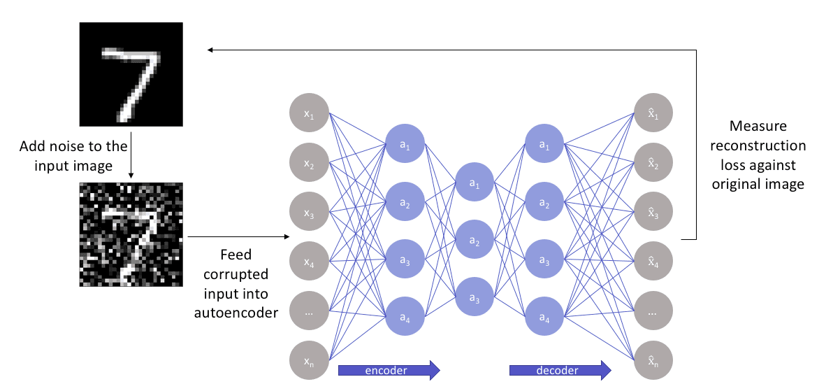
The denoising autoencoder gets rid of noise by learning a representation of the input where the noise can be filtered out easily.

While removing noise directly from the image seems difficult, the autoencoder performs this by mapping the input data into a lower-dimensional manifold (like in undercomplete autoencoders), where filtering of noise becomes much easier.

Essentially, denoising autoencoders work with the help of non-linear dimensionality reduction. The loss function generally used in these types of networks is L2 or L1 loss.

5. Variational autoencoders

Standard and variational autoencoders learn to represent the input just in a compressed form called the latent space or the bottleneck.

Therefore, the latent space formed after training the model is not necessarily continuous and, in effect, might not be easy to interpolate.

For example—

This is what a variational autoencoder would learn from the input:

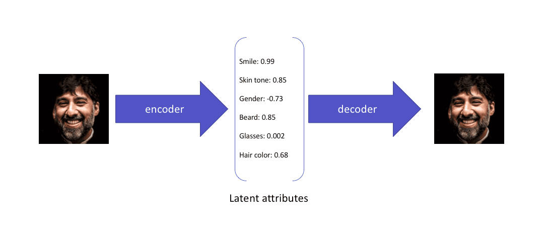
While these attributes explain the image and can be used in reconstructing the image from the compressed latent space, they do not allow the latent attributes to be expressed in a probabilistic fashion.

Variational autoencoders deal with this specific topic and express their latent attributes as a probability distribution, leading to the formation of a continuous latent space that can be easily sampled and interpolated.

When fed the same input, a variational autoencoder would construct latent attributes in the following manner:

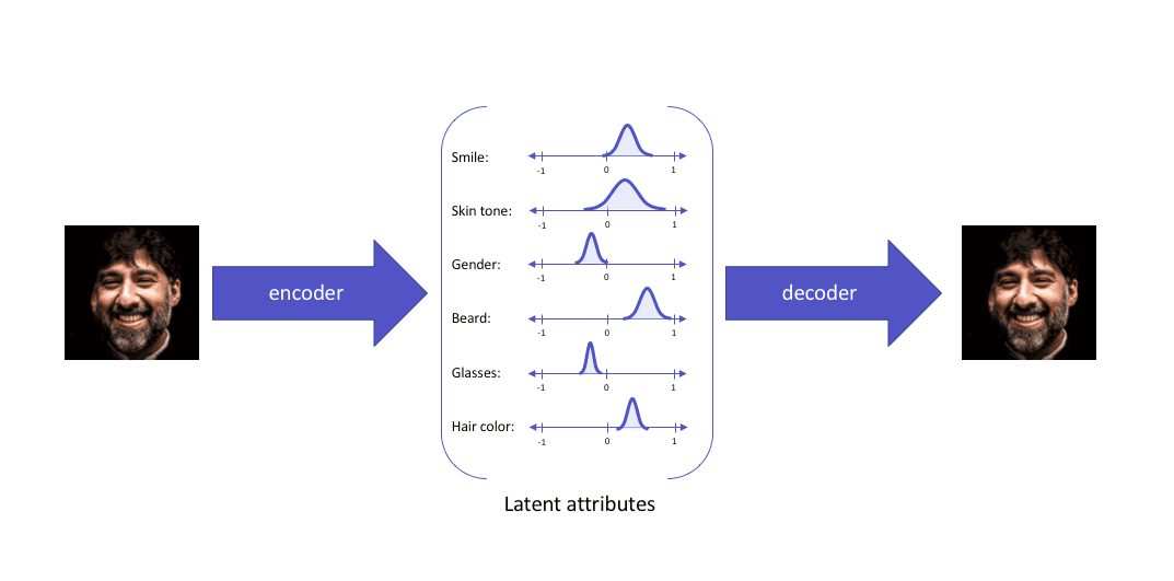
Variational autoencoder constructing latent attributes

The latent attributes are then sampled from the latent distribution formed and fed to the decoder, reconstructing the input.

The motivation behind expressing the latent attributes as a probability distribution can be very easily understood via statistical expressions.

Here’s how this works—

We aim at identifying the characteristics of the latent vector z that reconstructs the output given a particular input. Effectively, we want to study the characteristics of the latent vector given a certain output x[p(z|x)].

While estimating the distribution becomes impossible mathematically, a much simpler and easier option is to build a parameterized model that can estimate the distribution for us. It does it by minimizing the KL divergence between the original distribution and our parameterized one.

Expressing the parameterized distribution as q, we can infer the possible latent attributes used in the image reconstruction.

Assuming the prior z to be a multivariate Gaussian model, we can build a parameterized distribution as one containing two parameters, the mean and the variance. The corresponding distribution is then sampled and fed to the decoder, which then proceeds to reconstruct the input from the sample points.

But—

While this seems easy in theory, it becomes impossible to implement because backpropagation cannot be defined for a random sampling process performed before feeding the data to the decoder.

To get by this hurdle, we use the reparameterization trick—a cleverly defined way to bypass the sampling process from the neural network.

What is it all about?

In the reparameterization trick, we randomly sample a valueε from a unit Gaussian and then scale this by the latent distribution varianceσ and shift it by the mean μ of the same.

Now, we have left behind the sampling process as something done outside what the backpropagation pipeline handles, and the sampled value ε acts just like another input to the model, that is fed at the bottleneck.

A diagrammatic view of what we attain can be expressed as:

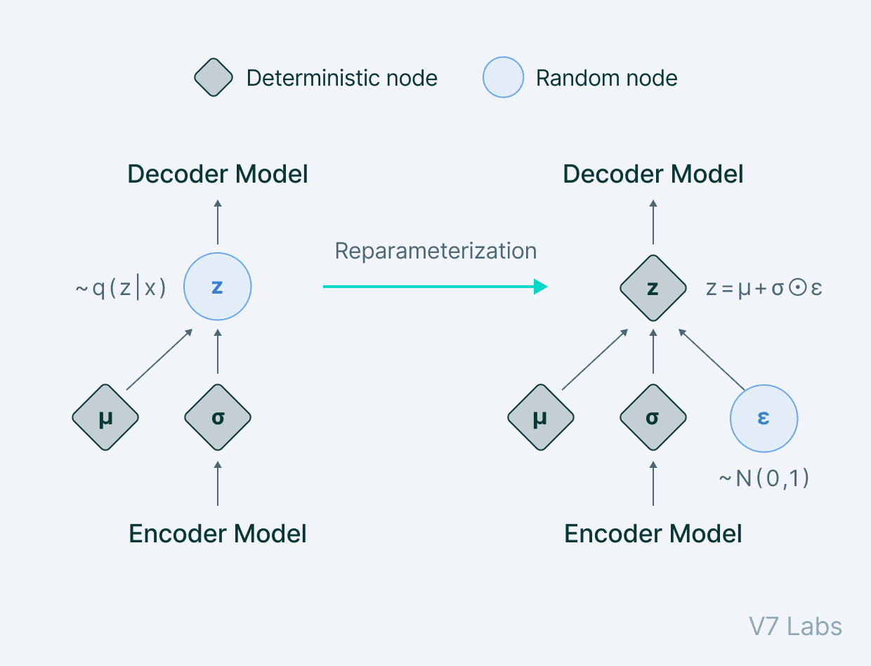
The variational autoencoder thus allows us to learn smooth latent state representations of the input data.

To train a VAE, we use two loss functions: the reconstruction loss and the other being the KL divergence.

While reconstruction loss enables the distribution to correctly describe the input, by focusing only on minimizing the reconstruction loss, the network learns very narrow distributions—akin to discrete latent attributes.

The KL divergence loss prevents the network from learning narrow distributions and tries to bring the distribution closer to a unit normal distribution.

The summarised loss function can be expressed as:

‍

L = |x - \hat{x}| + β \sum_{i} K L (q_{j} (z | x) ∥ N (0, 1))

‍

Where N denotes the normal unit distribution and $β$ denotes a weighting factor.

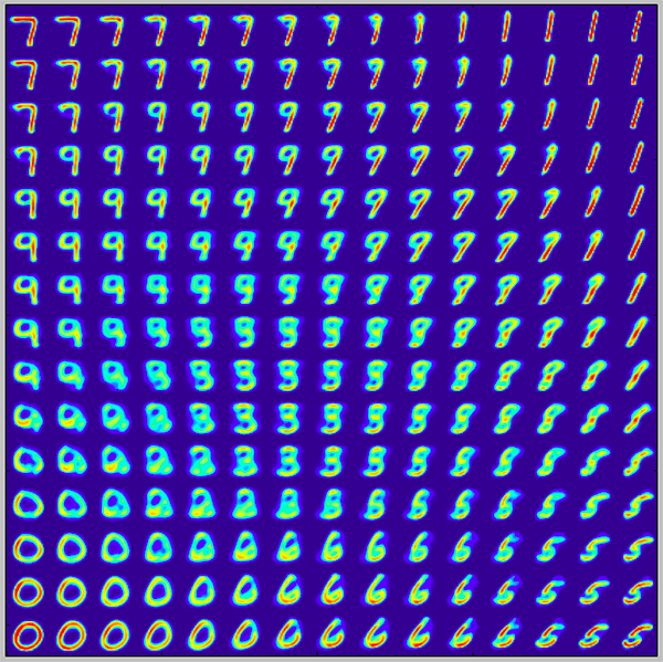
The primary use of variational autoencoders can be seen in generative modeling.

Sampling from the latent distribution trained and feeding the result to the decoder can lead to data being generated in the autoencoder.

A sample of MNIST digits generated by training a variational autoencoder is shown below:

Applications of autoencoders

Now that you understand various types of autoencoders, let’s summarize some of their most common use cases.

1. Dimensionality reduction

Undercomplete autoencoders are those that are used for dimensionality reduction.

These can be used as a pre-processing step for dimensionality reduction as they can perform fast and accurate dimensionality reductions without losing much information.

Furthermore, while dimensionality reduction procedures like PCA can only perform linear dimensionality reductions, undercomplete autoencoders can perform large-scale non-linear dimensionality reductions.

2. Image denoising

Autoencoders like the denoising autoencoder can be used for performing efficient and highly accurate image denoising.

Unlike traditional methods of denoising, autoencoders do not search for noise, they extract the image from the noisy data that has been fed to them via learning a representation of it. The representation is then decompressed to form a noise-free image.

Denoising autoencoders thus can denoise complex images that cannot be denoised via traditional methods.

3. Generation of image and time series data

Variational Autoencoders can be used to generate both image and time series data.

The parameterized distribution at the bottleneck of the autoencoder can be randomly sampled to generate discrete values for latent attributes, which can then be forwarded to the decoder,leading to generation of image data. VAEs can also be used to model time series data like music.

💡 Pro tip: Check out a recent application of VAEs in the domain of musical tone generation.

4. Anomaly detection

Undercomplete autoencoders can also be used for anomaly detection.

For example—consider an autoencoder that has been trained on a specific dataset P. For any image sampled for the training dataset, the autoencoder is bound to give a low reconstruction loss and is supposed to reconstruct the image as is.

For any image which is not present in the training dataset, however, the autoencoder cannot perform the reconstruction, as the latent attributes are not adapted for the specific image that has never been seen by the network.

As a result, the outlier image gives off a very high reconstruction loss and can easily be identified as an anomaly with the help of a proper threshold.

Autoencoders in a nutshell: Key takeaways

Well, that was a lot to take in. Let’s do a quick recap of everything you've learned in this guide:

An autoencoder is an unsupervised learning technique for neural networks that learns efficient data representations (encoding) by training the network to ignore signal “noise.”
Autoencoders can be used for image denoising, image compression, and, in some cases, even generation of image data.
While autoencoders might seem easy at the first glance (as they have a very simple theoretical background), making them learn a representation of the input that is meaningful is quite difficult.
Autoencoders like the undercomplete autoencoder and the sparse autoencoder do not have large scale applications in computer vision compared to VAEs and DAEs which are still used in works since being proposed in 2013 (by Kingmaet al).

💡 Read next:

The Ultimate Guide to Object Detection

A Gentle Introduction to Image Segmentation for Machine Learning

The Beginner's Guide to Deep Reinforcement Learning

The Complete Guide to CVAT—Pros & Cons

5 Alternatives to Scale AI

YOLO: Real-Time Object Detection Explained

Domain Adaptation in Computer Vision: Everything You Need to Know

‍