F1 Score in Machine Learning: Intro & Calculation

Since the last decade, deep learning algorithms have been the number one choice for solving complex computer vision problems.

The capabilities of any algorithm are gauged by a set of evaluation metrics, the most popular one being model accuracy. For a long time, accuracy was the only metric used for comparing machine learning models.

However, accuracy only computes how many times a model made a correct prediction across the entire dataset, which remains valid if the dataset is class-balanced.

F1 score is an alternative machine learning evaluation metric that assesses the predictive skill of a model by elaborating on its class-wise performance rather than an overall performance as done by accuracy. F1 score combines two competing metrics- precision and recall scores of a model, leading to its widespread use in recent literature.

In this article, we’ll dig deeper into the F1 score. Here’s what we’ll cover:

• What is F1 Score?
• How to calculate F1 Score?
• How to compute F measures with Python?

Looking for other machine learning guides? Take a look here:

• What Is Computer Vision? [Basic Tasks & Techniques]
• An Introductory Guide to Quality Training Data for Machine Learning
• 65+ Best Free Datasets for Machine Learning

What is F1 score?

F1 score is a machine learning evaluation metric that measures a model’s accuracy. It combines the precision and recall scores of a model.

The accuracy metric computes how many times a model made a correct prediction across the entire dataset. This can be a reliable metric only if the dataset is class-balanced; that is, each class of the dataset has the same number of samples.

Nevertheless, real-world datasets are heavily class-imbalanced, often making this metric unviable. For example, if a binary class dataset has 90 and 10 samples in class-1 and class-2, respectively, a model that only predicts “class-1,” regardless of the sample, will still be 90% accurate. Accuracy computes how many times a model made a correct prediction across the entire dataset. However, can this model be called a good predictor? This is where the F1 score comes into play.

We will look into the mathematical explanation behind the metric in the next section, but let’s first understand the precision and recall in relation to a binary class dataset with classes labeled “positive” and “negative.”

Precision measures how many of the “positive” predictions made by the model were correct.

Recall measures how many of the positive class samples present in the dataset were correctly identified by the model.

Precision and recall offer a trade-off, i.e., one metric comes at the cost of another. More precision involves a harsher critic (classifier) that doubts even the actual positive samples from the dataset, thus reducing the recall score. On the other hand, more recall entails a lax critic that allows any sample that resembles a positive class to pass, which makes border-case negative samples classified as “positive,” thus reducing the precision. Ideally, we want to maximize both precision and recall metrics to obtain the perfect classifier.

The F1 score combines precision and recall using their harmonic mean, and maximizing the F1 score implies simultaneously maximizing both precision and recall. Thus, the F1 score has become the choice of researchers for evaluating their models in conjunction with accuracy.

💡Pro tip: Need to brush up on Precision vs. Recall? Check out our guide.

How to calculate F1 score?

To understand the calculation of the F1 score, we first need to look at a confusion matrix.

A confusion matrix represents the predictive performance of a model on a dataset. For a binary class dataset (which consists of, suppose, “positive” and “negative” classes), a confusion matrix has four essential components:

1. True Positives (TP): Number of samples correctly predicted as “positive.”
2. False Positives (FP): Number of samples wrongly predicted as “positive.”
3. True Negatives (TN): Number of samples correctly predicted as “negative.”
4. False Negatives (FN): Number of samples wrongly predicted as “negative.”

Using the components of the confusion matrix, we can define the various metrics used for evaluating classifiers—accuracy, precision, recall, and F1 score.

The F1 score is defined based on the precision and recall scores, which are mathematically defined as follows:

The F1 score is calculated as the harmonic mean of the precision and recall scores, as shown below. It ranges from 0-100%, and a higher F1 score denotes a better quality classifier.

Why is the F1 score calculated using the harmonic mean instead of simple arithmetic or geometric means? To put it simply: the harmonic mean encourages similar values for precision and recall. That is, the more the precision and recall scores deviate from each other, the worse the harmonic mean. A more detailed, mathematical explanation can be found here.

In terms of the basic four elements of the confusion matrix, by replacing the expressions for precision and recall scores in the equation above, the F1 score can also be written as follows:

For calculating the F1 scores of a multi-class dataset, a one-vs-all technique is used to compute the individual scores for every class in the dataset. The harmonic mean for the class-wise precision and recall values are taken. The net F1 score is then calculated using different averaging techniques, which we shall look at next.

Macro-averaged F1 Score

The macro-averaged F1 score of a model is just a simple average of the class-wise F1 scores obtained. Mathematically, it is expressed as follows (for a dataset with “n” classes):

The macro-averaged F1 score is useful only when the dataset being used has the same number of data points in each of its classes. However, most real-world datasets are class imbalanced—different categories have different amounts of data. In such cases, a simple average may be a misleading performance metric.

Micro-averaged F1 score

The micro-averaged F1 score is a metric that makes sense for multi-class data distributions. It uses “net” TP, FP, and FN values for calculating the metric.

The net TP refers to the sum of the class-wise TP scores of a dataset, which are calculated by dissolving a confusion matrix into one-vs-all matrices corresponding to each class.

If we have a confusion matrix, let’s say “M,” such that “M_ij” indicates the element for the ith row and jth column, the micro F1 score can be mathematically expressed as follows:

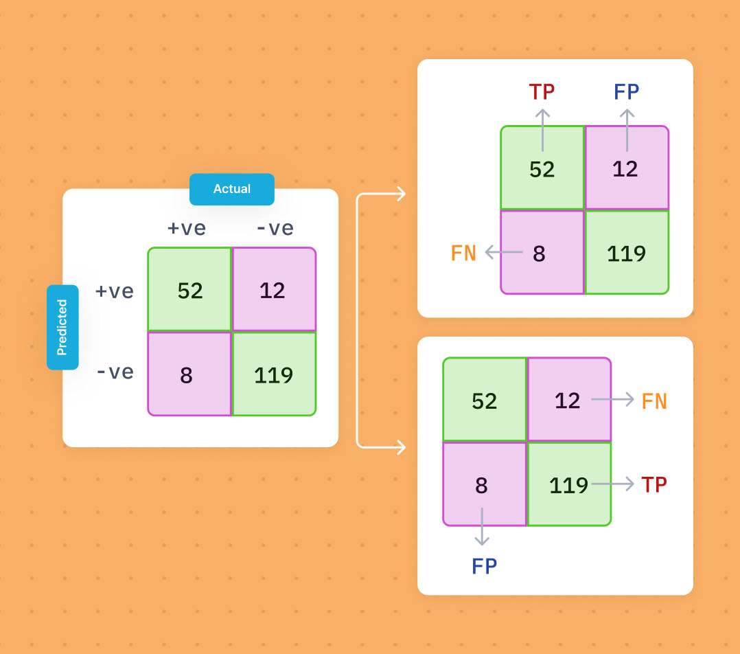
For a binary class dataset, a micro F1 score is simply the accuracy score. Let us understand why it is so. Consider an exemplar confusion matrix as shown below.

When the positive class is considered, the FP is 12, and the FN is 8. However, for the negative class, the initial FP and FN switch places. The FP is now 8, and the FN is 12. So, mathematically the micro F1 score becomes:

In the final step, the TP, TN, FP, and FN represent the original definitions of the components of a confusion matrix that we have talked about at the beginning of this section.

Sample-weighted F1 score

The sample-weighted F1 score is ideal for computing the net F1 score for class-imbalanced data distribution. As the name suggests, it is a weighted average of the class-wise F1 scores, the weights of which are determined by the number of samples available in that class.

For an “N”-class dataset, the sample-weighted F1 score is simply:

Where,

An example case demonstrating the weighted average F1-score is shown in the example below.

The obtained sample-weighted F1 score has also been juxtaposed with the macro F1 score, which is the simple average of the class-wise scores. Since the class imbalance is insignificant in this example (240 and 260 samples in the positive and negative classes, respectively), the deviation between the macro and the weighted scores is not significant either. However, the deviation will increase in larger datasets with more drastic class imbalances.

Fβ score

The Fβ score is a generalized version of the F1 score. It computes the harmonic mean, just like an F1 score, but with a priority given to either precision or recall. “β” represents the weighting coefficient (a hyperparameter set by the user, which is always greater than 0). Mathematically, it is represented as follows:

We talk about the F1 score in cases where β is 1. A β value greater than 1 favors the recall metric, while values lower than 1 favor the precision metric. F0.5 and F2 are the most commonly used measures other than F1 scores.

The Fβ score is useful when we want to prioritize one measure while preserving results from the other measure.

For example, in the case of COVID-19 detection, False Negative results are detrimental—since a COVID positive patient is diagnosed as COVID negative, leading to the spread of the disease. In this case, the F2 measure is more useful to minimize the False Negatives while also trying to keep the precision score as high as possible. In other cases, it might be necessary to reduce the False Positives, where a lower β value (like an F0.5 score) is desired.

How to compute F measures in Python?

The F1 score can be calculated easily in Python using the “f1_score” function of the scikit-learn package. The function takes three arguments (and a few others which we can ignore for now) as its input: the true labels, the predicted labels, and an “average” parameter which can be binary/micro/macro/weighted/none.

The “binary” mode of the average parameter is used to get the class-specific F1 score for a binary-class dataset. As the name suggests, the micro, macro, and weighted averages are the corresponding averaging schemes for calculating the scores on the datasets with any number of classes. Using “None” returns all the individual class-wise F1 scores. An example usage of the function is shown below.

To get a more comprehensive list of the metrics all at once, the “classification_report” function of scikit-learn can be used. It takes the true and predicted labels as inputs and outputs the class-wise metrics as well as the different average metrics.

The Fβ score can be computed in Python using the “fbeta_score” function, much like the f1_score function we saw above, with the additional “beta” input argument. An example with different β values is shown below:

Key takeaways

For a long time, accuracy has been the metric of choice for evaluating machine learning models.

However, it provides very little insight into the finer workings of a model, especially in real-world datasets where we do not have sufficient control over the data sampling. A fair evaluation of model performance is as critical as designing a problem-specific model architecture.

The F1 score is a much more comprehensive evaluation metric in comparison since it maximizes two competing objectives—the precision and recall scores—simultaneously. F1 score can be used for both class-wise and overall evaluations. Furthermore, the other variations of the F1 score, specifically the Fβ score, allow controlling the F score metric based on the problem at hand by prioritizing the minimization of either false positive or false negative losses.

Different averaging techniques are used to compute the overall F1 score of datasets like micro, macro, and sample averaged F scores. The class-wise and global F1 score metrics can be easily computed with Python, the most popular language for machine learning, making it one of the most used metrics in classification performance evaluation.