First up, regression metrics. Regression metrics are used to evaluate the performance of algorithms that predict continuous numerical values. Let’s go through the most important regression metrics.
Mean Absolute Error (MAE) is a popular metric used to evaluate the performance of regression models in machine learning and statistics. It measures the average magnitude of errors between predicted and actual values without considering their direction. MAE is especially useful in applications that aim to minimize the average error and is less sensitive to outliers than other metrics like Mean Squared Error (MSE).
Given a dataset with n observations, where $y_i$ is the actual value and $ŷ_i$ is the predicted value for the i-th data point in the dataset, the Mean Absolute Error (MAE) can be calculated using the following formula:
$$\mathrm{MAE} = \frac{1}{{\mathrm{n}}}\sum_{}{\mathrm{y}} - {\mathrm{ŷ}}$$
Here, the absolute difference between each actual value $(y)$ and its corresponding predicted value $(ŷ)$ is calculated, and the sum of these absolute differences is divided by the total number of observations $(n)$ to obtain the average error.
The strength of MAE lies in its ability to provide an intuitive and easily interpretable measure of model performance. A lower MAE indicates a better model fit, showing that the model's predictions are, on average, closer to the true values. It is beneficial when comparing different models on the same dataset, as it can help identify the model with the most accurate predictions.
MAE measures the average magnitude of errors in the predictions made by the model (without considering their direction).
Use MAE when you want a simple, interpretable metric to evaluate the performance of your regression model.
Avoid using MAE to emphasize the impact of larger errors, as it does not penalize them heavily.
import torch
# Create tensors for actual and predicted values
actual_values = torch.tensor([2.0, 4.0, 6.0, 8.0])
predicted_values = torch.tensor([2.5, 3.5, 6.5, 7.5])
def mean_absolute_error(y_true, y_pred):
# Calculate the absolute difference between actual and predicted values
abs_diff = torch.abs(y_true - y_pred)
# Calculate the mean of the absolute differences
mae = torch.mean(abs_diff)
return mae
# Calculate MAE
mae = mean_absolute_error(actual_values, predicted_values)
print(f"Mean Absolute Error: {mae:.2f}")import torch
# Create tensors for actual and predicted values
actual_values = torch.tensor([2.0, 4.0, 6.0, 8.0])
predicted_values = torch.tensor([2.5, 3.5, 6.5, 7.5])
def mean_absolute_error(y_true, y_pred):
# Calculate the absolute difference between actual and predicted values
abs_diff = torch.abs(y_true - y_pred)
# Calculate the mean of the absolute differences
mae = torch.mean(abs_diff)
return mae
# Calculate MAE
mae = mean_absolute_error(actual_values, predicted_values)
print(f"Mean Absolute Error: {mae:.2f}")Mean Squared Error (MSE) is another widely used metric for assessing the performance of regression models in machine learning and statistics. It measures the average squared difference between the predicted and actual values, thus emphasizing larger errors. MSE is particularly useful in applications where the goal is to minimize the impact of outliers or when the error distribution is assumed to be Gaussian.
Gaussian distribution, is a probability distribution that is symmetric about the mean, showing that data near the mean are more frequent in occurrence than data far from the mean
Given a dataset with n observations, where y_i is the actual value and ŷ_i is the predicted value for the i-th observation, the Mean Squared Error (MSE) can be calculated using the following formula:
$$\mathrm{MSE} = \frac{1}{{\mathrm{n}}}\sum_{{\mathrm{i}} = 1}^{{\mathrm{n}}}({\mathrm{Y}}_{{\mathrm{i}}} - \widehat{{\mathrm{Y}}}_{{\mathrm{i}}})^2$$
Here, the squared difference between each actual value $(y_i)$ and its corresponding predicted value $(ŷ_i)$ is calculated, and the sum of these squared differences is divided by the total number of observations $(n)$ to obtain the average squared error.
MSE provides a measure of model performance that penalizes larger errors more severely than smaller ones. A lower MSE indicates a better model fit, demonstrating that the model's predictions are, on average, closer to the true values. It is commonly used when comparing different models on the same dataset, as it can help identify the model with the most accurate predictions.
MSE measures the average squared difference between the actual and predicted values, penalizing larger errors more heavily than smaller ones.
Use MSE when you want to place a higher emphasis on larger errors.
Avoid using MSE if you need an easily interpretable metric or if your dataset has a lot of outliers, as it can be sensitive to them.
import torch
# Create tensors for actual and predicted values
actual_values = torch.tensor([2.0, 4.0, 6.0, 8.0])
predicted_values = torch.tensor([2.5, 3.5, 6.5, 7.5])
def mean_squared_error(y_true, y_pred):
# Calculate the squared difference between actual and predicted values
squared_diff = (y_true - y_pred) ** 2
# Calculate the mean of the squared differences
mse = torch.mean(squared_diff)
return mse
# Calculate MSE
mse = mean_squared_error(actual_values, predicted_values)
print(f"Mean Squared Error: {mse:.2f}")import torch
# Create tensors for actual and predicted values
actual_values = torch.tensor([2.0, 4.0, 6.0, 8.0])
predicted_values = torch.tensor([2.5, 3.5, 6.5, 7.5])
def mean_squared_error(y_true, y_pred):
# Calculate the squared difference between actual and predicted values
squared_diff = (y_true - y_pred) ** 2
# Calculate the mean of the squared differences
mse = torch.mean(squared_diff)
return mse
# Calculate MSE
mse = mean_squared_error(actual_values, predicted_values)
print(f"Mean Squared Error: {mse:.2f}")The Mean Squared Error (MSE) square root measures the average squared difference between the predicted and actual values. Root Mean Squared Error (RMSE) has the same unit as the target variable, making it more interpretable and easier to relate to the problem context than MSE.
Given a dataset with n observations, where $y_i$ is the actual value, and $ŷ_i$ is the predicted value for the i-th observation, the Root Mean Squared Error (RMSE) can be calculated using the following formula:
$$\mathrm{RMSE} = \sqrt{\frac{\sum_{{\mathrm{i}} = 1}^{{\mathrm{N}}}{\mathrm{y}}({\mathrm{i}}) - {\mathrm{ŷ}}({\mathrm{i}})^2}{{\mathrm{n}}}}$$
Here, the squared difference between each actual value (y_i) and its corresponding predicted value (ŷ_i) is calculated, and the sum of these squared differences is divided by the total number of observations (n) to obtain the average squared error. The square root of this value is then taken to compute the RMSE.
RMSE can provide a measure of model performance that balances the emphasis on larger errors (as in MSE) with interpretability (since it has the same unit as the target variable). A lower RMSE indicates a better model fit, showing that the model's predictions are, on average, closer to the true values. It is commonly used when comparing different models on the same dataset, as it can help identify the model with the most accurate predictions.
Use RMSE to penalize larger errors and obtain a metric with the same unit as the target variable.
Avoid using RMSE if you need an interpretable metric or if your dataset has a lot of outliers.
import torch
# Create tensors for actual and predicted values
actual_values = torch.tensor([2.0, 4.0, 6.0, 8.0])
predicted_values = torch.tensor([2.5, 3.5, 6.5, 7.5])
def root_mean_squared_error(y_true, y_pred):
# Calculate the squared difference between actual and predicted values
squared_diff = (y_true - y_pred) ** 2
# Calculate the mean of the squared differences
mse = torch.mean(squared_diff)
# Take the square root of the mean squared error to obtain RMSE
rmse = torch.sqrt(mse)
return rmse
# Calculate RMSE
rmse = root_mean_squared_error(actual_values, predicted_values)
print(f"Root Mean Squared Error: {rmse:.2f}")import torch
# Create tensors for actual and predicted values
actual_values = torch.tensor([2.0, 4.0, 6.0, 8.0])
predicted_values = torch.tensor([2.5, 3.5, 6.5, 7.5])
def root_mean_squared_error(y_true, y_pred):
# Calculate the squared difference between actual and predicted values
squared_diff = (y_true - y_pred) ** 2
# Calculate the mean of the squared differences
mse = torch.mean(squared_diff)
# Take the square root of the mean squared error to obtain RMSE
rmse = torch.sqrt(mse)
return rmse
# Calculate RMSE
rmse = root_mean_squared_error(actual_values, predicted_values)
print(f"Root Mean Squared Error: {rmse:.2f}")
R Squared $(R^2)$, also known as the coefficient of determination, measures the proportion of the total variation in the target variable explained by the model's predictions.
$(R^2)$ ranges from 0 to 1, with higher values indicating a better model fit.
The significance of $(R^2)$ lies in its ability to provide an intuitive and easily interpretable measure of how well the model captures the underlying structure of the data.
It tells us the percentage of the variation in the target variable that the model's predictors can explain. $(R^2)$ is particularly useful when comparing different models on the same dataset, as it can help identify the model that best explains the variation in the target variable.
Given a dataset with n observations, where $y_i$ is the actual value, and $ŷ_i$ is the predicted value for the i-th observation, the R Squared can be calculated using the following formula:
$${\mathrm{r}} = \frac{{\mathrm{n}}(\sum_{}\mathrm{xy}) - (\sum_{}{\mathrm{x}})(\sum_{}{\mathrm{y}})}{\sqrt{{\mathrm{n}}\sum_{}{\mathrm{x}}^2 - (\sum_{}{\mathrm{x}})^2{\mathrm{n}}\sum_{}{\mathrm{y}}^2 - (\sum_{}{\mathrm{y}})^2}}$$
In this formula, the numerator represents the sum of the squared errors between the actual and predicted values (also known as the residual sum of squares). At the same time, the denominator represents the sum of the squared differences between the actual values and their mean (also known as the total sum of squares). These two quantities' ratios are subtracted from 1 to obtain the R-squared value.
R-squared measures the proportion of the variance in the dependent variable that the model's independent variables can explain.
Use R-squared when you want to understand how well your model is explaining the variation in the target variable compared to a simple average.
Avoid using it if your model has a large number of independent variables or if it is sensitive to outliers.
import torch
# Create tensors for actual and predicted values
actual_values = torch.tensor([2.0, 4.0, 6.0, 8.0])
predicted_values = torch.tensor([2.5, 3.5, 6.5, 7.5])
def r_squared_error(y_true, y_pred):
# Calculate the mean of the actual values
y_mean = torch.mean(y_true)
# Calculate the sum of squares (numerator)
residual_sum_of_squares = torch.sum((y_true - y_pred) ** 2)
# Calculate the total sum of squares (denominator)
total_sum_of_squares = torch.sum((y_true - y_mean) ** 2)
# Calculate R² using the formula
r_squared = 1 - (residual_sum_of_squares / total_sum_of_squares)
return r_squared
# Calculate R²
r_squared = r_squared_error(actual_values, predicted_values)
print(f"R Squared Error: {r_squared:.2f}")import torch
# Create tensors for actual and predicted values
actual_values = torch.tensor([2.0, 4.0, 6.0, 8.0])
predicted_values = torch.tensor([2.5, 3.5, 6.5, 7.5])
def r_squared_error(y_true, y_pred):
# Calculate the mean of the actual values
y_mean = torch.mean(y_true)
# Calculate the sum of squares (numerator)
residual_sum_of_squares = torch.sum((y_true - y_pred) ** 2)
# Calculate the total sum of squares (denominator)
total_sum_of_squares = torch.sum((y_true - y_mean) ** 2)
# Calculate R² using the formula
r_squared = 1 - (residual_sum_of_squares / total_sum_of_squares)
return r_squared
# Calculate R²
r_squared = r_squared_error(actual_values, predicted_values)
print(f"R Squared Error: {r_squared:.2f}")Classification metrics assess the performance of machine learning models for classification tasks. They aim to assign an input data point to one of several predefined categories.
Let’s go through the most commonly used classification metrics.
Pro tip: Already building your classification model? Check out our guides on image classification and video classification.
Accuracy is a fundamental evaluation metric for assessing the overall performance of a classification model. It is the ratio of the correctly predicted instances to the total instances in the dataset. The formula for calculating accuracy is:
$$\mathrm{Accuracy} = \frac{\mathrm{TP} + \mathrm{TN}}{\mathrm{TP} + \mathrm{FP} + \mathrm{TN} + \mathrm{FN}}$$
Accuracy measures the proportion of correct predictions made by the model out of all predictions.
Accuracy is useful when the class distribution is balanced, and false positives and negatives have equal importance.
If the dataset is imbalanced or the cost of false positives and negatives differs, accuracy may not be an appropriate metric.
A confusion matrix, also known as an error matrix, is a tool used to evaluate the performance of classification models in machine learning and statistics. It presents a summary of the predictions made by a classifier compared to the actual class labels, allowing for a detailed analysis of the classifier's performance across different classes.
The confusion matrix provides a comprehensive view of the model's performance, including each class's correct and incorrect predictions.
It helps identify misclassification patterns and calculate various evaluation metrics such as precision, recall, F1-score, and accuracy. By analyzing the confusion matrix, you can diagnose the model's strengths and weaknesses and improve its performance.

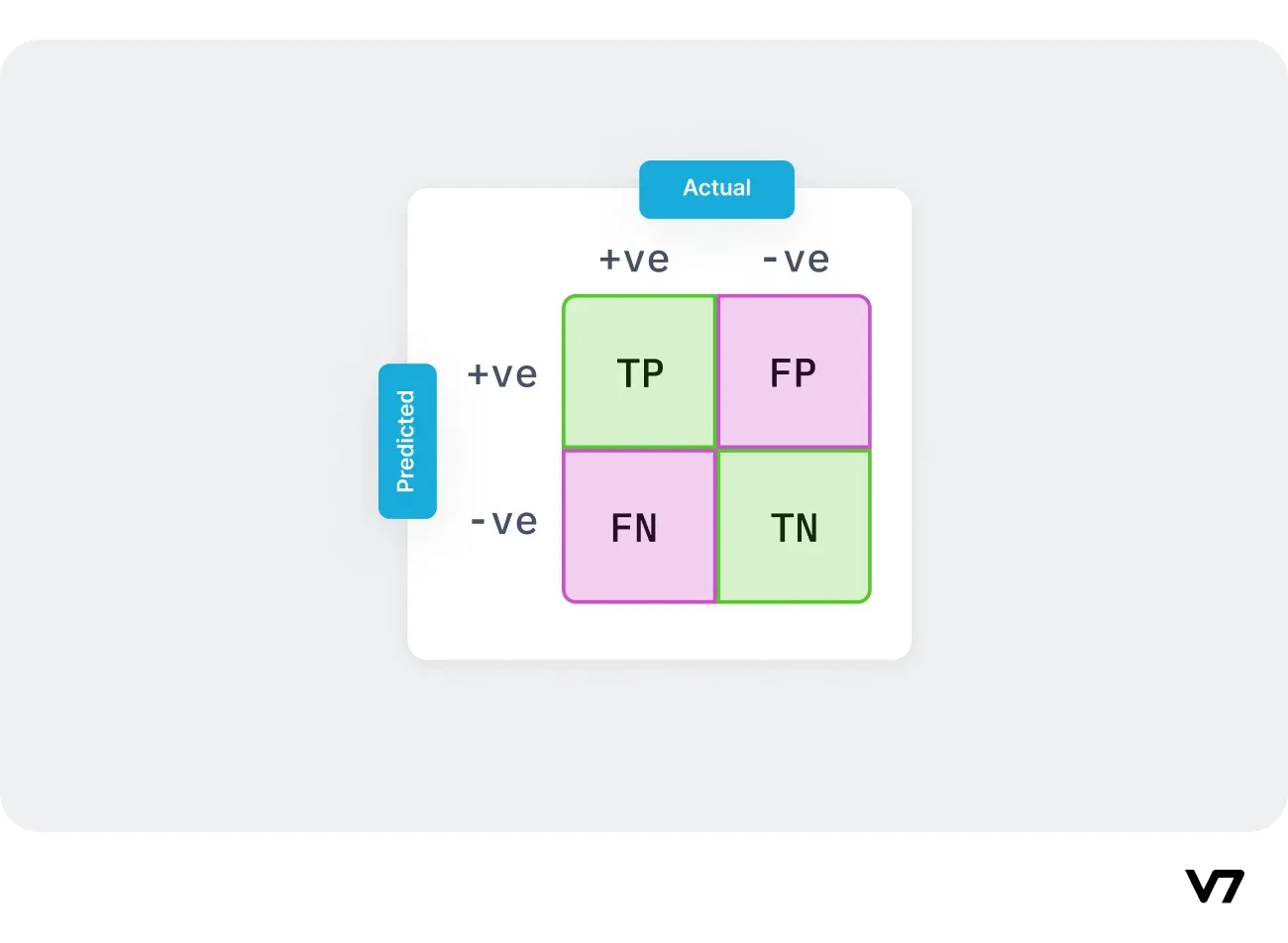
Let's start with an example confusion matrix for a binary classifier (though it can easily be extended to the case of more than two classes):
Two possible predicted classes are "yes" and "no." If we were predicting the presence of a disease in a patient, for example, "yes" would mean they have the disease, and "no" would mean they don't. The classifier made a total of 165 predictions (e.g., 165 patients were being tested for the presence of that disease). Of those 165 cases, the classifier predicted "yes" 110 times and "no" 55 times. In reality, 105 patients in the sample have the disease, and 60 patients do not.
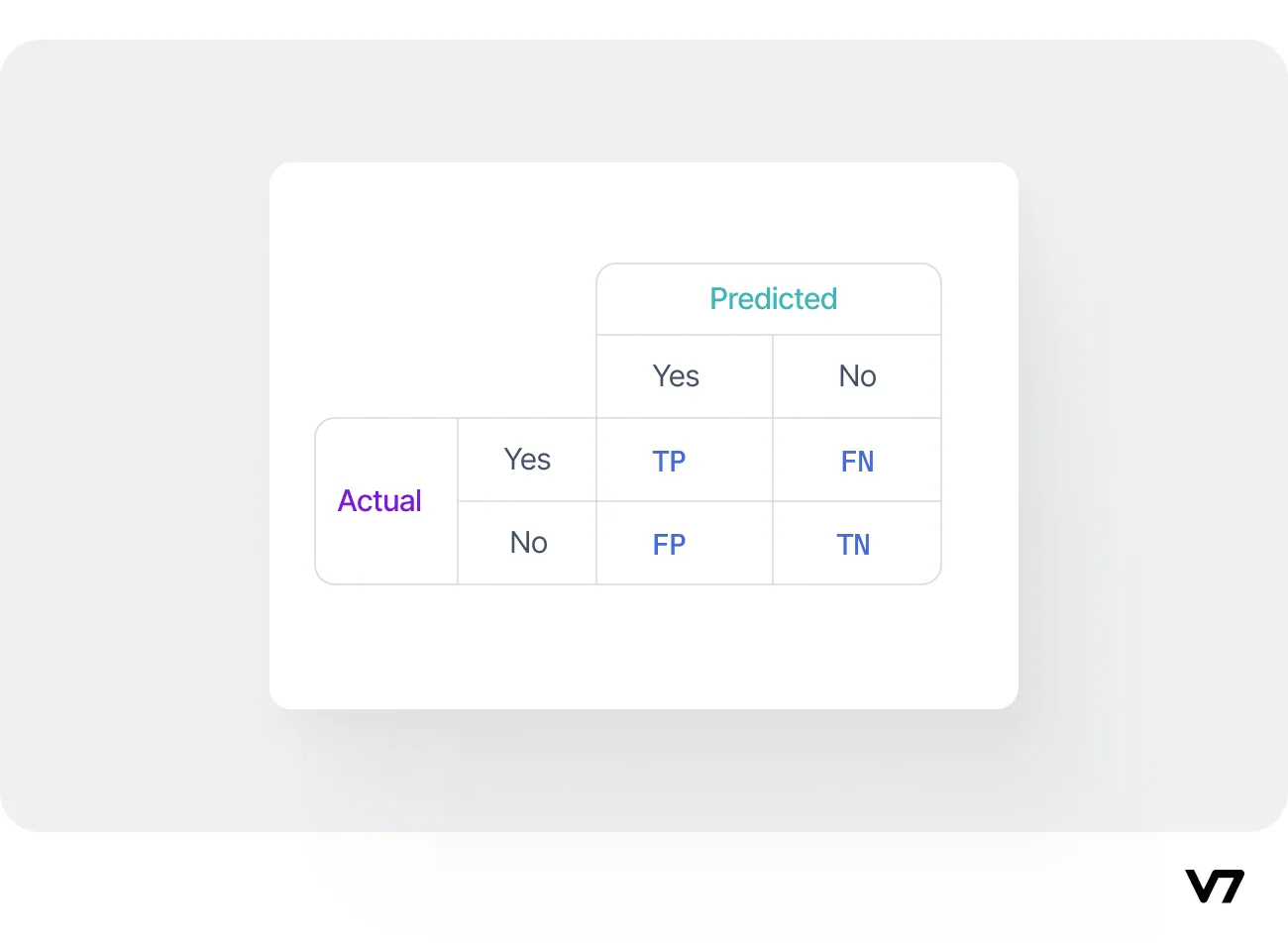
Let's create a confusion matrix in the given disease classification case and interpret it.
Here's the confusion matrix:

TP: True Positives - The number of patients with the disease correctly predicted as "yes."
TN: True Negatives - The number of patients without the disease was correctly predicted as "no."
FP: False Positives - The number of patients who don't have the disease but were incorrectly predicted as "yes."
FN: False Negatives - The number of patients who have the disease but were incorrectly predicted as "no."
From the given information:
Total predictions = 165
Predicted "yes" = 110
Predicted "no" = 55
Actual "yes" = 105
Actual "no" = 60
To fill in the confusion matrix, we need to find the values of TP, TN, FP, and FN. We can't determine these values from the information given, so let's assume we have those values:

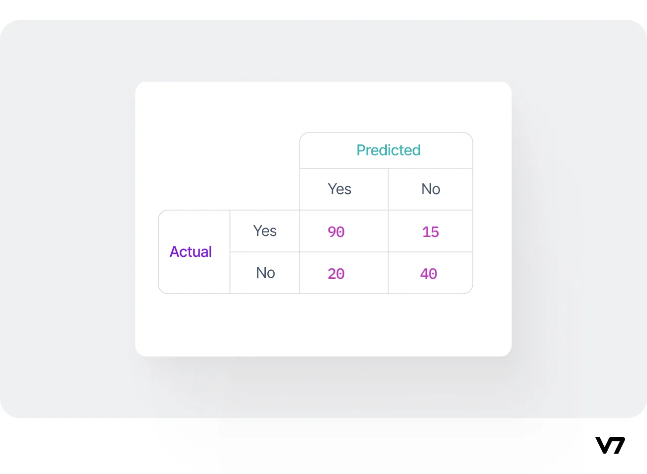
From this confusion matrix, we can interpret the following:
TP (90): Out of 105 patients with the disease, the model correctly predicted "yes" for 90 patients.
FN (15): The model incorrectly predicted "no" for 15 patients with the disease.
FP (20): Out of 60 patients without the disease, the model incorrectly predicted "yes" for 20 patients.
TN (40): The model correctly predicted "no" for 40 patients who don't have the disease.
The confusion matrix provides a detailed breakdown of the model's performance, allowing us to identify specific types of errors.
Use a confusion matrix when you want to visualize the performance of a classification model and analyze the types of errors it makes.
import torch
def confusion_matrix(true_labels, pred_labels, num_classes):
"""
Calculate the confusion matrix for a classification task.
Args:
true_labels (torch.Tensor): Ground truth labels.
pred_labels (torch.Tensor): Predicted labels from the model.
num_classes (int): Number of classes in the classification task.
Returns:
torch.Tensor: The confusion matrix of shape (num_classes, num_classes).
"""
assert true_labels.shape == pred_labels.shape, "Shape mismatch between true_labels and pred_labels"
cm = torch.zeros(num_classes, num_classes, dtype=torch.int64)
for t, p in zip(true_labels.view(-1), pred_labels.view(-1)):
cm[t.long(), p.long()] += 1
return cm
# Assuming you have true_labels and pred_labels tensors
# true_labels = ...
# pred_labels = ...
num_classes = 4 # Number of classes in your classification task
cm = confusion_matrix(true_labels, pred_labels, num_classes)
print(cm)import torch
def confusion_matrix(true_labels, pred_labels, num_classes):
"""
Calculate the confusion matrix for a classification task.
Args:
true_labels (torch.Tensor): Ground truth labels.
pred_labels (torch.Tensor): Predicted labels from the model.
num_classes (int): Number of classes in the classification task.
Returns:
torch.Tensor: The confusion matrix of shape (num_classes, num_classes).
"""
assert true_labels.shape == pred_labels.shape, "Shape mismatch between true_labels and pred_labels"
cm = torch.zeros(num_classes, num_classes, dtype=torch.int64)
for t, p in zip(true_labels.view(-1), pred_labels.view(-1)):
cm[t.long(), p.long()] += 1
return cm
# Assuming you have true_labels and pred_labels tensors
# true_labels = ...
# pred_labels = ...
num_classes = 4 # Number of classes in your classification task
cm = confusion_matrix(true_labels, pred_labels, num_classes)
print(cm)Pro tip: Check out this in-depth guide about the confusion matrix
Precision and recall are essential evaluation metrics in machine learning for understanding the trade-off between false positives and false negatives.
$$\mathrm{\Pr ecision} = \frac{\mathrm{TP}}{\mathrm{TP} + \mathrm{FP}}$$
$$\mathrm{Recall} = \frac{\mathrm{TP}}{\mathrm{TP} + \mathrm{FN}}$$
Precision (P) is the proportion of true positive predictions among all positive pedictions. It is a measure of how accurate the positive predictions are.
Recall (R), also known as sensitivity or true positive rate (TPR), is the proportion of true positive predictions among all actual positive instances. It measures the classifier's ability to identify positive instances correctly.
A high precision means the model has fewer false positives, while a high recall means fewer false negatives. Depending on the specific problem you're trying to solve, you might prioritize one of these metrics over the other.
Imagine you're a detective trying to solve a crime in a city. Your task is to identify criminals from a list of suspects. You have to find the real criminals and minimize false accusations.
Let's think of your investigation in terms of machine learning. Your detective model makes predictions by classifying suspects as criminals or innocent. The model's performance can be measured by two key metrics: Precision and Recall.
Precision measures how well your detective model correctly identifies criminals without falsely accusing innocent people.
Let's say you've identified ten suspects as criminals. If seven are actual criminals, and three are innocent, your precision is 70% (7/10). High precision indicates that you're great at avoiding false accusations.
Now, let's talk about the recall.
The recall measures how well your detective model captures all the criminals in the city. It's like casting a wide net to ensure no criminals slip through the cracks.
Let's say there are a total of 20 criminals in the city. If you've identified seven, your recall is 35% (7/20). A high recall means you're excellent at catching criminals, even if some innocent people might get caught in the net.
In a perfect world, you would want to have both high precision and high recall, ensuring that you're accurate in your accusations and comprehensive in capturing all criminals. However, there's often a trade-off between the two metrics in practice: improving one may come at the cost of the other.

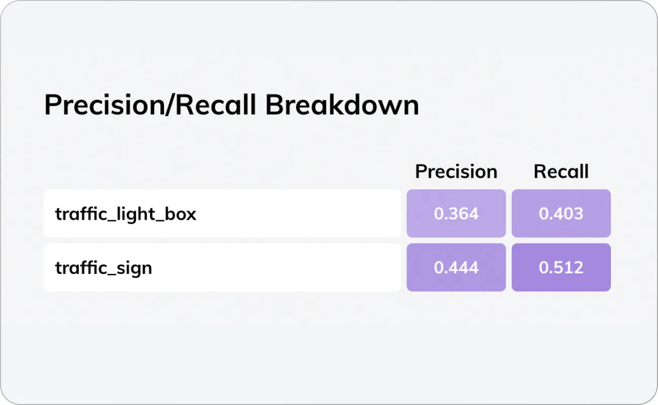
Precision/recall breakdown for a traffic light and sign detection model in V7
Precision measures the proportion of true positive predictions among all positive predictions, while recall measures the proportion of true positive predictions among all actual positive instances.
Precision and recall are useful when the class distribution is imbalanced or when the cost of false positives and false negatives is different.
Accuracy might be more appropriate if the dataset is balanced and the costs of false positives and negatives are equal.
import torch
def precision_recall(y_true, y_pred):
assert y_true.shape == y_pred.shape, "Input tensors must have the same shape"
# Convert predictions to binary (0 or 1) by applying a threshold (0.5 in this case)
y_pred_binary = (y_pred >= 0.5).float()
# Calculate True Positives (TP), False Positives (FP), and False Negatives (FN)
TP = torch.sum(y_true * y_pred_binary)
FP = torch.sum((1 - y_true) * y_pred_binary)
FN = torch.sum(y_true * (1 - y_pred_binary))
# Calculate Precision and Recall
precision = TP / (TP + FP)
recall = TP / (TP + FN)
return precision, recall
# Example usage
y_true = torch.tensor([1, 0, 1, 1, 0, 1])
y_pred = torch.tensor([0.9, 0.3, 0.7, 0.1, 0.2, 0.8])
precision, recall = precision_recall(y_true, y_pred)
print(f"Precision: {precision:.4f}, Recall: {recall:.4f}")import torch
def precision_recall(y_true, y_pred):
assert y_true.shape == y_pred.shape, "Input tensors must have the same shape"
# Convert predictions to binary (0 or 1) by applying a threshold (0.5 in this case)
y_pred_binary = (y_pred >= 0.5).float()
# Calculate True Positives (TP), False Positives (FP), and False Negatives (FN)
TP = torch.sum(y_true * y_pred_binary)
FP = torch.sum((1 - y_true) * y_pred_binary)
FN = torch.sum(y_true * (1 - y_pred_binary))
# Calculate Precision and Recall
precision = TP / (TP + FP)
recall = TP / (TP + FN)
return precision, recall
# Example usage
y_true = torch.tensor([1, 0, 1, 1, 0, 1])
y_pred = torch.tensor([0.9, 0.3, 0.7, 0.1, 0.2, 0.8])
precision, recall = precision_recall(y_true, y_pred)
print(f"Precision: {precision:.4f}, Recall: {recall:.4f}")Pro tip: Check out this comprehensive guide on Precision and Recall
The F1-score is the harmonic mean of precision and recall, providing a metric that balances both measures. It is beneficial when dealing with imbalanced datasets, where one class is significantly more frequent than the other. The formula for the F1 score is:
$${\mathrm{F}}1\mathrm{Score} = \frac{2}{\frac{1}{\mathrm{\Pr ecision}} + \frac{1}{\mathrm{Recall}}} = \frac{2{\mathrm{x}}\mathrm{\Pr ecision}{\mathrm{x}}\mathrm{Recall}}{\mathrm{\Pr ecision} + \mathrm{Recall}}$$
The significance of the F1 score lies in its ability to provide a harmonized assessment of a model's performance when both precision and recall are important. Unlike accuracy, which can be misleading in cases of class imbalance, the F1 score considers the balance between false positives and false negatives.
A high F1 score indicates that the model has a high precision (low false positives) and high recall (low false negatives), which is often desirable in various applications.
The F1-score is the harmonic mean of precision and recall, providing a metric that considers false positives and false negatives.
The F1-score is useful when the class distribution is imbalanced or when the cost of false positives and false negatives is different.
Accuracy might be more appropriate if the dataset is balanced and the costs of false positives and negatives are equal.
import torch
def f1_score(y_true, y_pred, eps=1e-8):
assert y_true.size() == y_pred.size(), "Input tensors should have the same size"
# Convert the predicted probabilities to binary predictions
y_pred_binary = torch.round(y_pred)
# Calculate True Positives, False Positives, and False Negatives
tp = torch.sum(y_true * y_pred_binary)
fp = torch.sum((1 - y_true) * y_pred_binary)
fn = torch.sum(y_true * (1 - y_pred_binary))
# Calculate Precision and Recall
precision = tp / (tp + fp + eps)
recall = tp / (tp + fn + eps)
# Calculate F1 Score
f1 = 2 * precision * recall / (precision + recall + eps)
return f1.item()
# Example usage
y_true = torch.tensor([1, 0, 1, 1, 0, 1], dtype=torch.float32)
y_pred = torch.tensor([0.9, 0.2, 0.8, 0.6, 0.3, 0.7], dtype=torch.float32)
f1 = f1_score(y_true, y_pred)
print(f"F1 Score: {f1}")import torch
def f1_score(y_true, y_pred, eps=1e-8):
assert y_true.size() == y_pred.size(), "Input tensors should have the same size"
# Convert the predicted probabilities to binary predictions
y_pred_binary = torch.round(y_pred)
# Calculate True Positives, False Positives, and False Negatives
tp = torch.sum(y_true * y_pred_binary)
fp = torch.sum((1 - y_true) * y_pred_binary)
fn = torch.sum(y_true * (1 - y_pred_binary))
# Calculate Precision and Recall
precision = tp / (tp + fp + eps)
recall = tp / (tp + fn + eps)
# Calculate F1 Score
f1 = 2 * precision * recall / (precision + recall + eps)
return f1.item()
# Example usage
y_true = torch.tensor([1, 0, 1, 1, 0, 1], dtype=torch.float32)
y_pred = torch.tensor([0.9, 0.2, 0.8, 0.6, 0.3, 0.7], dtype=torch.float32)
f1 = f1_score(y_true, y_pred)
print(f"F1 Score: {f1}")Pro tip: Check out this guide on F1 Score and its fundamentals.
The AU-ROC is a popular evaluation metric for binary classification problems. It measures the model's ability to distinguish between positive and negative classes. The ROC curve plots the true positive rate (recall) against the false positive rate (1 - specificity) at various classification thresholds. The AU-ROC represents the area under the ROC curve, and a higher value indicates better model performance.
The significance of the AU-ROC lies in its ability to provide a comprehensive view of a model's performance across all possible classification thresholds. It considers the trade-off between true positive rate (TPR) and false positive rate (FPR) and quantifies the classifier's ability to differentiate between the two classes.
A higher AU-ROC value indicates better performance, with a perfect classifier having an AU-ROC of 1 and a random classifier having an AU-ROC of 0.5.
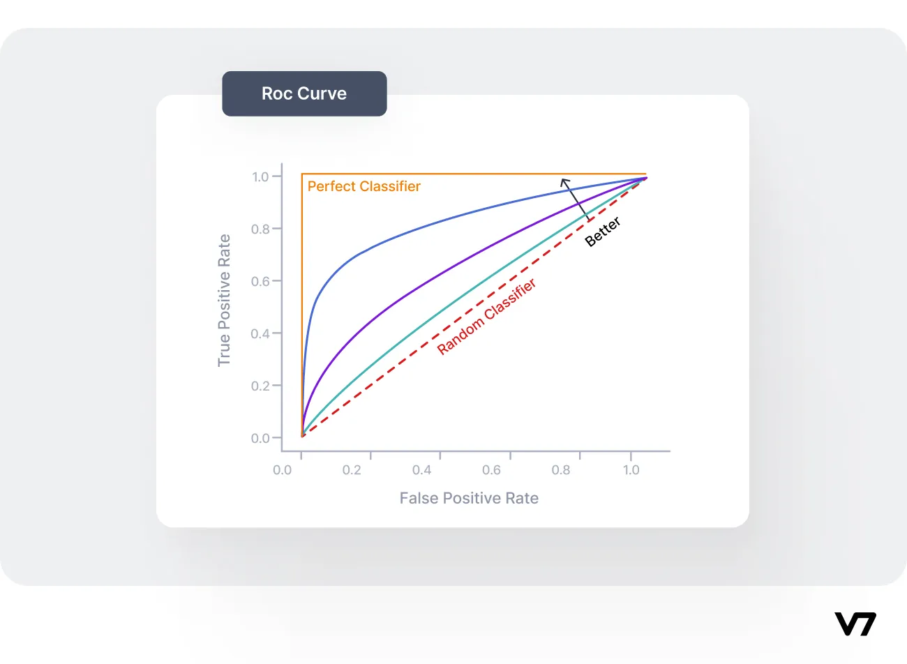
Source: ROC Curve
AU-ROC represents the model's ability to discriminate between positive and negative classes. A higher AU-ROC value indicates better classification performance.
Use AU-ROC to compare the performance of different classification models, especially when the class distribution is imbalanced.
Accuracy might be more appropriate if the dataset is balanced and the costs of false positives and negatives are equal.
import torch
import numpy as np
from sklearn.metrics import roc_auc_score
# Assuming you have the following PyTorch tensors:
# - `y_true`: a 1D tensor containing the true binary labels (0 or 1) for each sample
# - `y_pred`: a 1D tensor containing the predicted probabilities for the positive class
# Convert tensors to NumPy arrays
y_true_np = y_true.detach().cpu().numpy()
y_pred_np = y_pred.detach().cpu().numpy()
# Calculate AUROC score using scikit-learn
auroc = roc_auc_score(y_true_np, y_pred_np)
print(f"AUROC score: {auroc}")import torch
import numpy as np
from sklearn.metrics import roc_auc_score
# Assuming you have the following PyTorch tensors:
# - `y_true`: a 1D tensor containing the true binary labels (0 or 1) for each sample
# - `y_pred`: a 1D tensor containing the predicted probabilities for the positive class
# Convert tensors to NumPy arrays
y_true_np = y_true.detach().cpu().numpy()
y_pred_np = y_pred.detach().cpu().numpy()
# Calculate AUROC score using scikit-learn
auroc = roc_auc_score(y_true_np, y_pred_np)
print(f"AUROC score: {auroc}")In this example, we first convert the PyTorch tensors y_true and y_pred into NumPy arrays. Then, we use the roc_auc_score function from scikit-learn to calculate the AU-ROC score. Note that y_true should contain binary labels (0 or 1), and y_pred should contain the predicted probabilities for the positive class.
Let’s discuss other important metrics widely used in object detection and segmentation tasks. Intersection over Union (IoU) and mean Average Precision (mAP) help assess the performance of models that identify and localize multiple objects within images.
Intersection over Union (IoU) is a popular evaluation metric in object detection and segmentation tasks. It measures the overlap between the predicted bounding box and the ground truth bounding box, providing an understanding of how well the model detects objects in images. The IoU is calculated as the ratio of the intersection area to the union area of the two bounding boxes:

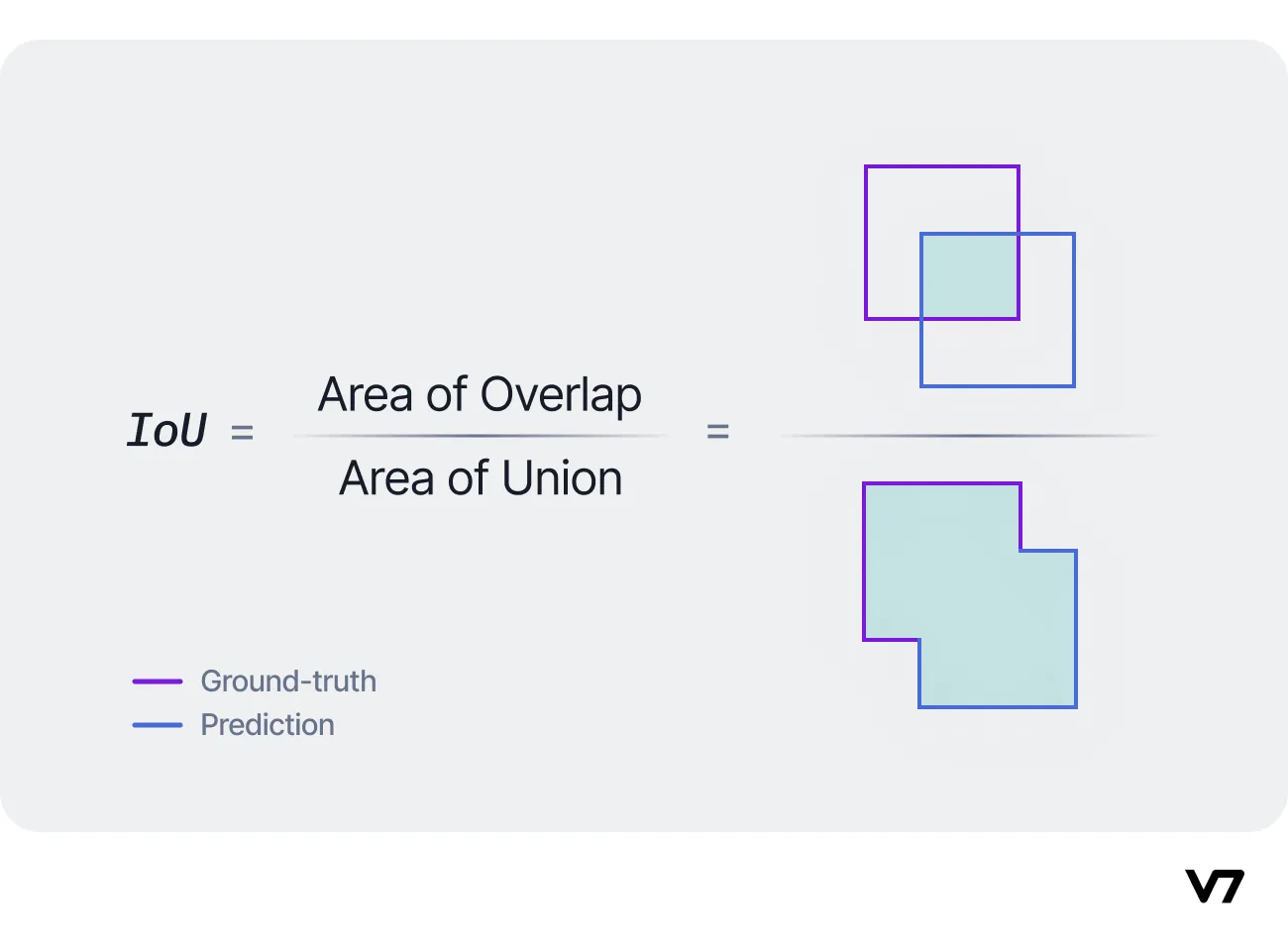
A higher IoU value indicates a better model performance, with 1.0 being the perfect score.
IoU quantifies how well the model's predictions align with the ground truth bounding boxes.
Use IoU for object detection and segmentation tasks.
IoU is irrelevant for classification or regression.
import torch
def bbox_iou(box1, box2):
# Calculate the coordinates of the intersection rectangle
x1 = torch.max(box1[0], box2[0])
y1 = torch.max(box1[1], box2[1])
x2 = torch.min(box1[2], box2[2])
y2 = torch.min(box1[3], box2[3])
# Calculate the area of the intersection rectangle
intersection_area = (x2 - x1).clamp(0) * (y2 - y1).clamp(0)
# Calculate the area of both input boxes
box1_area = (box1[2] - box1[0]) * (box1[3] - box1[1])
box2_area = (box2[2] - box2[0]) * (box2[3] - box2[1])
# Calculate the area of the union of both boxes
union_area = box1_area + box2_area - intersection_area
# Calculate the IoU
iou = intersection_area / union_area
return iou
# Example usage
box1 = torch.tensor([50, 50, 150, 150], dtype=torch.float32)
box2 = torch.tensor([100, 100, 200, 200], dtype=torch.float32)
iou = bbox_iou(box1, box2)
print("IoU:", iou)import torch
def bbox_iou(box1, box2):
# Calculate the coordinates of the intersection rectangle
x1 = torch.max(box1[0], box2[0])
y1 = torch.max(box1[1], box2[1])
x2 = torch.min(box1[2], box2[2])
y2 = torch.min(box1[3], box2[3])
# Calculate the area of the intersection rectangle
intersection_area = (x2 - x1).clamp(0) * (y2 - y1).clamp(0)
# Calculate the area of both input boxes
box1_area = (box1[2] - box1[0]) * (box1[3] - box1[1])
box2_area = (box2[2] - box2[0]) * (box2[3] - box2[1])
# Calculate the area of the union of both boxes
union_area = box1_area + box2_area - intersection_area
# Calculate the IoU
iou = intersection_area / union_area
return iou
# Example usage
box1 = torch.tensor([50, 50, 150, 150], dtype=torch.float32)
box2 = torch.tensor([100, 100, 200, 200], dtype=torch.float32)
iou = bbox_iou(box1, box2)
print("IoU:", iou)Mean Average Precision (mAP) is another widely used performance metric in object detection and segmentation tasks. It is the average of the precision values calculated at different recall levels, providing a single value that captures the overall effectiveness of the model. The mAP can be computed using the following steps:
1. Calculate each class's average precision (AP) using the precision-recall curve. Average Precision is the area under the PR curve for a single query or class. It can be calculated using the following steps:
Interpolate the precision values: For each recall level, find the highest precision value with recall equal to or greater than the current recall level. This step ensures that the precision values are monotonically decreasing from left to right.
Calculate AP: Compute the area under the interpolated PR curve by summing the product of the change in recall and interpolated precision at each recall level: AP = Sum(P(i) * (R(i) - R(i-1)))
2. Calculate the mean of the AP values across all classes:
$$\mathrm{mAP} = \frac{1}{{\mathrm{n}}}\sum_{{\mathrm{k}} = 1}^{{\mathrm{k}} = {\mathrm{n}}}AP_{{\mathrm{k}}}$$
Where $AP_k$ is the average precision for the k-th query or class, and $N$ is the total number of queries or classes.
Mean Average Precision (mAP) is a metric that computes the average precision (AP) for multiple object classes. It combines precision and recall, considering the presence of false positives and false negatives and their distribution across different confidence thresholds. The mAP score ranges from 0 (worst performance) to 1 (best performance).
Use mAP in object detection and segmentation tasks to evaluate the model's overall performance across all object classes—when there are multiple object classes, and you want a single metric to assess the model's performance across all classes.
Avoid using mAP when you need a detailed analysis of the model's performance in specific classes, as it averages the performance across all classes. In such cases, analyze class-wise AP instead.
import torch
def calculate_iou(prediction_box, ground_truth_box):
"""
Calculate the Intersection over Union (IoU) of two bounding boxes.
"""
x1 = max(prediction_box[0], ground_truth_box[0])
y1 = max(prediction_box[1], ground_truth_box[1])
x2 = min(prediction_box[2], ground_truth_box[2])
y2 = min(prediction_box[3], ground_truth_box[3])
intersection_area = max(x2 - x1, 0) * max(y2 - y1, 0)
prediction_box_area = (prediction_box[2] - prediction_box[0]) * (prediction_box[3] - prediction_box[1])
ground_truth_box_area = (ground_truth_box[2] - ground_truth_box[0]) * (ground_truth_box[3] - ground_truth_box[1])
union_area = prediction_box_area + ground_truth_box_area - intersection_area
return intersection_area / union_area
def calculate_map(predictions, ground_truths, num_classes, iou_threshold=0.5):
"""
Calculate the mean Average Precision (mAP) for multiple object classes.
"""
aps = []
for c in range(num_classes):
# Get predictions and ground truth for the current class
predictions_class = [p for p in predictions if p[1] == c]
ground_truths_class = [g for g in ground_truths if g[1] == c]
# Sort predictions by confidence score
predictions_class.sort(key=lambda x: x[2], reverse=True)
true_positives = torch.zeros(len(predictions_class))
false_positives = torch.zeros(len(predictions_class))
# Mark true positives and false positives
for i, pred in enumerate(predictions_class):
iou_max = -1
gt_match = -1
for j, gt in enumerate(ground_truths_class):
iou = calculate_iou(pred[0], gt[0])
if iou > iou_max:
iou_max = iou
gt_match = j
if iou_max >= iou_threshold:
if not ground_truths_class[gt_match][2]:
true_positives[i] = 1
ground_truths_class[gt_match][2] = True
else:
false_positives[i] = 1
else:
false_positives[i] = 1
# Compute Precision and Recall
tp_cumsum = torch.cumsum(true_positives, dim=0)
fp_cumsum = torch.cumsum(false_positives, dim=0)
precision = tp_cumsum / (tp_cumsum + fp_cumsum)
recall = tp_cumsum / len(ground_truths_class)
# Compute Average Precision
ap = 0
for t in torch.arange(0, 1.1, 0.1):
if torch.sum(recall >= t) == 0:
p = 0
else:
p = torch.max(precision[recall >= t])
ap += p / 11
aps.append(ap)
# Compute mean Average Precision
map = sum(aps) / len(aps)
return mapimport torch
def calculate_iou(prediction_box, ground_truth_box):
"""
Calculate the Intersection over Union (IoU) of two bounding boxes.
"""
x1 = max(prediction_box[0], ground_truth_box[0])
y1 = max(prediction_box[1], ground_truth_box[1])
x2 = min(prediction_box[2], ground_truth_box[2])
y2 = min(prediction_box[3], ground_truth_box[3])
intersection_area = max(x2 - x1, 0) * max(y2 - y1, 0)
prediction_box_area = (prediction_box[2] - prediction_box[0]) * (prediction_box[3] - prediction_box[1])
ground_truth_box_area = (ground_truth_box[2] - ground_truth_box[0]) * (ground_truth_box[3] - ground_truth_box[1])
union_area = prediction_box_area + ground_truth_box_area - intersection_area
return intersection_area / union_area
def calculate_map(predictions, ground_truths, num_classes, iou_threshold=0.5):
"""
Calculate the mean Average Precision (mAP) for multiple object classes.
"""
aps = []
for c in range(num_classes):
# Get predictions and ground truth for the current class
predictions_class = [p for p in predictions if p[1] == c]
ground_truths_class = [g for g in ground_truths if g[1] == c]
# Sort predictions by confidence score
predictions_class.sort(key=lambda x: x[2], reverse=True)
true_positives = torch.zeros(len(predictions_class))
false_positives = torch.zeros(len(predictions_class))
# Mark true positives and false positives
for i, pred in enumerate(predictions_class):
iou_max = -1
gt_match = -1
for j, gt in enumerate(ground_truths_class):
iou = calculate_iou(pred[0], gt[0])
if iou > iou_max:
iou_max = iou
gt_match = j
if iou_max >= iou_threshold:
if not ground_truths_class[gt_match][2]:
true_positives[i] = 1
ground_truths_class[gt_match][2] = True
else:
false_positives[i] = 1
else:
false_positives[i] = 1
# Compute Precision and Recall
tp_cumsum = torch.cumsum(true_positives, dim=0)
fp_cumsum = torch.cumsum(false_positives, dim=0)
precision = tp_cumsum / (tp_cumsum + fp_cumsum)
recall = tp_cumsum / len(ground_truths_class)
# Compute Average Precision
ap = 0
for t in torch.arange(0, 1.1, 0.1):
if torch.sum(recall >= t) == 0:
p = 0
else:
p = torch.max(precision[recall >= t])
ap += p / 11
aps.append(ap)
# Compute mean Average Precision
map = sum(aps) / len(aps)
return mapPro tip: Check out this in-depth guide about Mean Average Precision
Selecting the appropriate performance metric is critical to building effective machine learning models and ensuring the success of your MLOps pipeline.
The choice of metric depends on various factors, including the project goals, business objectives, and the strengths and weaknesses of each metric. Here's a summary of deciding which metric to use for a given project:
Understand your project's primary goals and consider what aspects of the model's performance are most important. For instance, minimizing false negatives in a fraud detection system may be more critical than overall accuracy.
Align the metric choice with your organization's business objectives. For example, a retail company may prioritize precision in predicting customer churn, as it impacts marketing costs and customer retention strategies.
Familiarize yourself with the strengths and weaknesses of each metric to make an informed choice. For instance, accuracy can be misleading in imbalanced datasets, so if you know your data is not perfectly balanced, don’t go for this metric.
Choose metrics that are easily understandable and interpretable by stakeholders. A simpler metric, such as accuracy or precision, may be more suitable for communication purposes than more complex metrics like AU-ROC or mAP.
The choice of metric should be suitable for the specific task and the data distribution at hand. For example, use regression metrics like Mean Squared Error (MSE) or Mean Absolute Error (MAE) for regression tasks and classification metrics like Precision and Recall for binary classification problems.
When evaluating a classification model, it's important to consider the trade-offs between performance aspects, such as the balance between false positives and false negatives. Adjusting classification thresholds allows you to optimize your model for specific business needs. Choosing the right evaluation metric is closely related to setting appropriate thresholds since different metrics prioritize different aspects of the model's performance.
By selecting a metric that aligns with your specific goals, you can fine-tune the threshold to achieve the desired balance between false positives and false negatives, optimizing the model to meet your requirements.
To effectively compare different models and algorithms, selecting appropriate metrics that consider your specific problem and objectives is important. Consistent use of metrics across various models will help identify the best-performing model for your project.
For instance, Precision, Recall, and F1-score are suitable for imbalanced datasets or when the cost of false positives and false negatives is asymmetric. Choose the metric that aligns with your goals (e.g., minimizing false positives or negatives).
Different machine learning tasks require specific evaluation metrics. Regression tasks commonly use metrics such as Mean Squared Error (MSE), Root Mean Squared Error (RMSE), and R² (R-Squared). In contrast, classification tasks use metrics like Accuracy, Confusion Matrix, Precision and Recall, F1-score, and AU-ROC. Object detection and segmentation tasks rely on metrics like Intersection over Union (IoU) and Mean Average Precision (mAP).
Choosing the right metric for a given project requires a clear understanding of the project goals and business objectives. Different metrics prioritize different aspects of model performance, and selecting the most relevant metric ensures that the model is optimized to meet the project's specific needs.
Be aware of the strengths and weaknesses of each metric. For example, accuracy is a simple and intuitive metric for classification tasks but can be misleading for imbalanced datasets. Metrics like Precision, Recall, and F1-score may be more appropriate.
Consistently use the chosen metric across various models and algorithms to effectively compare their performance. Doing so lets you identify the best-performing model that aligns with your project goals and business objectives.