Knowledge work automation
19 min read
—


The most common mistake analysts make with an LBO model is treating it like a valuation model.
It isn't. A discounted cash flow model asks what a business is worth today given future cash flows. An LBO model asks something different: given what we're paying, what combination of leverage, operating performance, and exit multiple gets us to a 25% IRR? The orientation is explicitly backward. You start from the return requirement and work toward the entry price, not from intrinsic value toward a trading range.
That reframe matters because it changes how you read every output the model produces. A DCF tells you whether the price is right. An LBO model tells you whether the deal works at that price.
This article covers the full mechanics: the five structural components of a standard LBO model, what each one measures, and how experienced deal teams interpret the outputs. It also covers where practitioners actually spend their time before the model opens, and how AI agents are compressing that pre-model data work. For context on the documents that typically feed an LBO model, see our guide to reading a Confidential Information Memorandum.
In this article:
What an LBO model is and how it differs from a DCF
The five structural components and what each one measures
What makes a company a good LBO target
How to read sensitivity tables like a practitioner
Where the real bottleneck in deal analysis sits, and what AI does about it

AI for document processing
Go from CIM to model without the manual extraction
Get started today
What an LBO model is (and what it isn't)
The LBO model is a returns calculator. That distinction changes everything about how you build it and everything about how you read it.
The model does not ask whether a company is fairly valued. It asks: at this price, with this debt structure, and these operating assumptions, what return does the equity investor earn at exit? Where a DCF anchors around a discount rate and works forward to an intrinsic value, an LBO anchors around a required return and works backward to test whether an entry price is achievable. A deal that produces a 28% IRR in the model is not necessarily a well-priced business. It means the specific combination of entry price, projected EBITDA growth, leverage, and exit multiple happens to produce a 28% annualised equity return.
Change any one of those inputs and the return changes. The model tells you the implications of your assumptions. It does not tell you which assumptions are correct.
Most LBO models are built in Excel and structured around a five-to-seven year hold. They are transaction-specific: unlike a DCF, which can be run in isolation, an LBO model only produces meaningful output once an entry price is assumed. You cannot run an LBO model on a company without first deciding what you would pay for it.
In practice, PE firms use LBO models at two distinct stages. The first is the screening stage: a simplified "paper LBO" run on publicly available financials to decide whether a target warrants further diligence. The second is the full diligence model, built after receiving the CIM and management accounts, which forms the basis of investment committee submissions and credit committee presentations. Most of the scrutiny on assumptions, particularly on entry EBITDA normalisation and exit multiple defensibility, happens at the second stage.
LBO vs. DCF: what actually differs in practice
Both use projected cash flows. That is where the structural similarity ends.
A DCF is a valuation exercise: project future free cash flows, apply a discount rate, and solve for present value. The output is an intrinsic value range. PE investors use DCFs alongside LBO models not to validate the LBO's return assumptions, but to check whether the entry price is defensible on a standalone valuation basis.
The LBO is a transaction exercise: assume an entry price, structure debt against it, project cash flows over the hold period, and solve for the equity return at exit. The output is an IRR and MoIC. If the IRR clears the fund's hurdle rate across a range of reasonable scenarios, the deal is investable at that price. If it only clears the hurdle under optimistic assumptions, the entry price needs to come down.
This is why PE analysts run both models on the same target but read them differently. A DCF that implies a company is worth $110M doesn't mean you should pay $110M for it in an LBO context. It means the valuation is defensible. Whether the deal works at $110M depends entirely on what leverage, operating assumptions, and exit thesis you're underwriting.
The five components of an LBO model
Every LBO model is built from the same five blocks. The sophistication sits in the quality of the inputs, not the architecture.
Extracting clean financial inputs from a CIM is the most time-consuming step in LBO analysis. AI compresses it.
1. Entry assumptions and sources and uses
Entry enterprise value is expressed as a multiple of EBITDA. In US middle-market buyouts, entry multiples commonly fall between 7x and 11x, though software businesses with high recurring revenue and healthcare services companies regularly trade above 12x, according to GF Data's quarterly M&A transaction surveys. Entry EV equals EBITDA times the entry multiple. From there, an equity bridge adjusts for net debt, working capital normalizations, and transaction fees to arrive at the equity contribution.
The sources and uses table captures what happens at close. Sources include senior secured debt (term loan, revolving credit facility), any subordinated or mezzanine debt, and sponsor equity. For a standard mid-market platform deal, debt typically represents 55 to 65% of total capitalization. Uses include the acquisition price, transaction fees (legal, financial advisory, financing costs), and any cash needed to refinance existing target debt.
The leverage multiple, calculated as total debt divided by EBITDA, is the key credit metric at this stage. Most bank lenders price middle-market debt at 4.5x to 5.5x leverage for a well-covered business. Anything above 6x requires a demonstrably defensive credit profile with contracted, recurring revenue.
2. The debt schedule
The debt schedule tracks how debt gets paid down over the hold period. It is where much of the equity value creation actually originates.
Post-acquisition, free cash flow generated by the business is applied against the outstanding debt. This is the cash sweep: each year, excess free cash flow reduces the debt balance after mandatory scheduled amortization. As the debt balance falls and enterprise value rises with EBITDA growth, equity value grows from both directions simultaneously.
This dynamic is why FCF conversion rate matters so much in LBO underwriting. A business that converts 65% of EBITDA to free cash flow can retire 30 to 40% of its initial debt load over five years with no operational improvement. A business that converts only 25%, due to heavy maintenance capex or working capital intensity, deleverages slowly and relies much more on EBITDA growth to generate equity value.
The debt schedule also captures covenant architecture: leverage ratio tests, interest coverage requirements, and distribution restrictions that govern the business throughout the hold. A well-built LBO model shows covenant headroom year by year. A covenant breach three years into the hold is typically more damaging to returns than a below-plan exit, because it triggers lender intervention and often forces a sale or recapitalisation at a disadvantageous time.
3. Financial projections
The projection section covers three to seven years of operating performance: revenue growth, EBITDA margin expansion or compression, capital expenditure, changes in working capital, and D&A. These inputs drive the free cash flow that services debt and ultimately delivers equity value at exit.
Base case projections in an LBO are consistently more conservative than management's own plan. A sponsor modelling 8% annual revenue growth in a business where management projects 15% is making a considered judgment about what the credit committee will accept, what the LP base will believe, and what the deal can survive if execution falls short.
The most contested number in the projection section is normalised EBITDA at entry. Add-backs are standard: one-time legal costs, executive compensation above market rate, non-recurring restructuring charges, facility relocation costs. Each add-back increases the presented EBITDA, which reduces the apparent entry multiple. A business acquired at "9x EBITDA" often works out to 11x or 12x true run-rate EBITDA when add-backs are scrutinised and reversed by a buyer's diligence team.
The EBITDA bridge is therefore the most analytically important artefact produced before the model opens. It requires reading the full financial statements, cross-referencing audited accounts against management account adjustments, and making a judgment call on which add-backs are genuinely non-recurring and which are recurring costs dressed up as one-offs. This judgment is irreducibly human. But getting to the point where that judgment can be exercised takes days of extraction work that AI now handles in minutes.
4. Exit assumptions
Exit enterprise value uses the same math as entry: projected EBITDA at exit times the exit multiple. The spread between entry and exit multiple is one of the most powerful drivers of equity return in any deal.
In a rising market, multiple expansion adds directly to equity value on top of operational improvement and debt paydown. In a compressed market, multiple contraction can erase years of solid operational execution. Conservative LBO models assume exit at the same multiple as entry. If the deal still clears the fund's hurdle rate at flat multiples, the return is structurally sound. If the model only works with expansion, the deal is partially a bet on market timing.
Common exit routes: secondary buyout sale to another PE sponsor, which is the most frequent outcome in middle-market deals; strategic acquisition by an industry buyer; IPO, which is less common outside large-cap; and dividend recapitalization. Each exit route affects timing assumptions and the distribution of proceeds back to LPs.
5. Returns: IRR and MoIC
Two metrics define the outcome, and they measure different things.
MoIC (Multiple on Invested Capital) is the total cash-on-cash return on equity. If a fund invests $45M of equity and distributes $160M at exit, the MoIC is 3.5x. Time is irrelevant to MoIC. A 3.5x over three years is a fundamentally different outcome from a 3.5x over eight years.
IRR (Internal Rate of Return) is the annualised equity return adjusted for the timing of cash flows. IRR rewards fast exits and penalises long holds. Two deals with identical MoIC can have very different IRRs depending on how the cash flows are distributed across the hold period.
PE fund target returns for middle-market buyouts typically sit around 20 to 25% gross IRR and 2.5 to 3.5x MoIC, according to Cambridge Associates' private equity benchmark data. A deal at 3.5x MoIC over a five-year hold implies a gross IRR of roughly 28 to 29%.
Hold period matters because PE funds have a finite life, typically ten years. A GP who holds a portfolio company for seven years before exit is consuming a disproportionate share of the fund's remaining life, compressing LP returns measured against capital returned per year of fund life.
The five levers of LBO equity return
Understanding why a deal produces the return it does requires decomposing the return into its drivers. There are five levers. Experienced investors routinely run this attribution on realised deals to understand which lever drove returns — and whether the thesis was correct or whether a good multiple covered for operational underperformance.
Entry multiple: the lower the entry price relative to EBITDA, the higher the potential return given all else equal. Entry multiple is largely set by market competition, but aggressive negotiation on EBITDA normalisation (stripping out add-backs that don't survive diligence) effectively reduces the entry multiple on a true run-rate basis.
Exit multiple: the most powerful single lever in most LBOs. A 2-turn multiple expansion from entry to exit adds roughly 20 to 30 percentage points of IRR for a typical mid-market deal, more than any other factor. This is also the least controllable lever, which is why conservative underwriting assumes flat multiples.
EBITDA growth: revenue growth and margin improvement compound over five to seven years and directly drive the exit enterprise value. This is where the operational value-creation thesis lives: pricing power, cost rationalisation, geographic expansion, add-on acquisitions.
Leverage: debt amplifies equity returns on the way up and amplifies losses on the way down. Higher initial leverage multiplies the equity return at exit given a fixed improvement in enterprise value, but it also reduces the buffer against operating headwinds and increases covenant risk.
Debt paydown: free cash flow that retires debt over the hold period increases equity value dollar for dollar at exit. A business that generates strong, consistent FCF contributes to returns through paydown even in a flat-multiple, flat-EBITDA scenario. This is the safest return driver of the five.
What makes a good LBO candidate
The debt structure of a leveraged buyout places specific demands on the business underneath it. Companies that don't meet those demands tend to produce covenant breaches rather than returns.
The most reliable LBO candidates share four characteristics.
Predictable, recurring free cash flow. Debt service is a fixed obligation. If the business has lumpy revenue, project-based contracts, or significant customer concentration, the debt schedule doesn't hold. Businesses with subscription revenue, long-term contracted income, or stable volume-based pricing: specialty distribution, B2B software with low churn, and outsourced services with multi-year contracts are structurally preferred because the FCF profile matches the debt service profile.
Defensible EBITDA margins. Thin margins leave no cushion. A business at 8% EBITDA margin under 5x leverage has almost no room for a revenue shortfall before the coverage ratio breaks. Mid-market buyouts typically target businesses with 15% or higher margins before they can support meaningful leverage.
A clear delevering path. This is about capex intensity and working capital characteristics as much as margin. An asset-light services business can convert more than 60% of EBITDA to free cash flow. A capital-intensive manufacturer with heavy maintenance requirements might convert 25 to 30%. Those businesses behave completely differently under the same debt load.
A defensible exit thesis. The entry IC memo should specify the expected exit route, the buyer universe, and the multiple range. A business with no obvious strategic buyers, limited secondary market interest, and poor public market comparables has a weak exit thesis regardless of operational performance.
Two sectors that consistently attract PE attention for these reasons are healthcare services and B2B software. Healthcare services businesses — clinic networks, speciality diagnostics, therapy practices — combine recurring patient volume, typically insurance-backed revenue, and fragmented ownership that supports add-on acquisition strategies. B2B software businesses with multi-year subscription contracts offer predictable ARR, low churn, and high incremental margins, which translate directly into strong FCF conversion and a natural exit market of both strategic buyers and larger PE platforms.
Sectors historically favoured for LBOs: healthcare services, B2B software with contractual revenue, professional services, industrial distribution, and specialty process chemicals. The common thread is contracted or recurring revenue, asset-light operations, and an established M&A buyer market at exit.
How to read sensitivity analysis outputs
A sensitivity table is not a valuation range. It is a map of how much room for error the deal has.
The most important sensitivity in any LBO model is the IRR matrix plotted across entry multiple and exit multiple. Each cell answers: if the fund pays X times EBITDA at entry and exits at Y times EBITDA, what return does equity earn? The target cell is where the base case lands. The question is how many adjacent cells also clear the hurdle rate.
A deal that achieves the target IRR only at the exact assumed entry and exit multiple is a deal with almost no margin of safety. A deal that achieves the target IRR across a wide band of entry and exit combinations is structurally more robust, regardless of which cell the base case occupies.

Sensitivity analysis should map outcomes across a realistic range of entry and exit assumptions, not a narrow band designed to make the base case look robust.
The second key sensitivity is EBITDA downside. At what EBITDA decline does the business breach its leverage covenant? At what decline does free cash flow no longer cover the interest obligation? These are floor tests that define how much operating risk the debt structure can absorb.
Experienced investors read sensitivity tables looking for the floor IRR, the return in the worst plausible scenario, rather than the base case. If the floor IRR is 14% on a fund with a 20% hurdle rate, the deal requires almost everything to go according to plan. That is a very different investment profile from one where the floor IRR is 21% and the base case is 29%.
The third sensitivity worth running on any deal is hold period. Most LBO models show IRR at the assumed exit year, but not across multiple exit years. Running IRR at year three, year four, five, six, and seven shows how quickly returns erode as the hold extends and how much of the base case depends on a timely exit.
One thing to verify when reviewing someone else's model: the sensitivity ranges. They should reflect realistic scenarios, not tight bands around the base case designed to make the deal look robust. If the sensitivity table shows EBITDA growth ranging from 9% to 12% for a business in a cyclical sector, those are not meaningful sensitivities. See our broader discussion of AI tools changing finance workflows for context on where automation is shifting analyst capacity in deal teams.


Where analysts actually lose time (and it isn't the model)
Ask any PE analyst what takes the most time on a new deal and the answer is never "building the model."
The model is the straightforward part. An experienced associate can build a standard five-year LBO in two to four hours once the inputs are clean. What takes days is what happens before any cell in the model is populated.
Reading the CIM to find the actual revenue figures: not the management-adjusted, re-segmented, normalised versions on the summary slides, but the raw reported numbers buried in the financial statements sixty pages in. Cross-referencing three years of historical EBITDA against audited financials that don't quite match the CIM presentation. Tracking down add-back justifications referenced in footnotes but not explained. Building a comparable transactions table by screening M&A databases for deals in the sector over the last five years. Structuring the debt stack based on current credit market conditions and where comparable credits have recently priced.
None of that is intellectually trivial. But most of it is data extraction, normalisation, and formatting. Not investment analysis.
A full CIM-to-first-pass-model workflow typically takes a two-person team two to three days before any real investment thesis discussion has happened. On a competitive process where management presentations are scheduled within the week, that timeline is a genuine constraint on how many deals a team can evaluate in parallel.
The manual CIM-to-model workflow requires five sequential steps before a return scenario can be run. AI agents compress the middle three.
How AI agents handle the CIM-to-LBO workflow
The most valuable thing AI has done for PE deal teams is not automate the model. It has compressed the data extraction and structuring work that comes before it.
V7 Go's CIM Review automation works from the source document directly. The agent reads the CIM, identifies and extracts revenue, EBITDA, and cash flow figures across all presented periods, normalises the adjustments, structures a sources and uses table based on the requested leverage parameters, builds a five-year projection using assumptions derived from the document's own market commentary and management plan, and produces a structured LBO output with entry enterprise value, debt schedule, IRR, and MoIC, with every figure cited back to its source page in the original document.
To illustrate: a case run through the CIM to LBO Report agent on a US-based mid-market battery materials recycler with approximately $45M revenue, roughly $9M reported EBITDA, and a CIM presenting three years of audited financials alongside a management projection.
The agent extracted the historical financials, identified and flagged two EBITDA add-backs (a one-time facility relocation cost and above-market management compensation), normalised EBITDA to approximately $9.86M, and structured a deal at 10x entry multiple. It modelled a five-year hold with a conservative revenue growth assumption, a standard leveraged capital structure, and an exit at the same multiple. The structured output: Entry EV $98.6M, total debt $53.2M, equity $45.4M, projected Exit EV $160.3M. MoIC 3.53x. IRR 28.7%.
The full output, covering transaction summary, debt schedule, five-year FCF model, and an annotated analysis with source citations, was available for analyst review before the team had finished reading the CIM's executive summary.
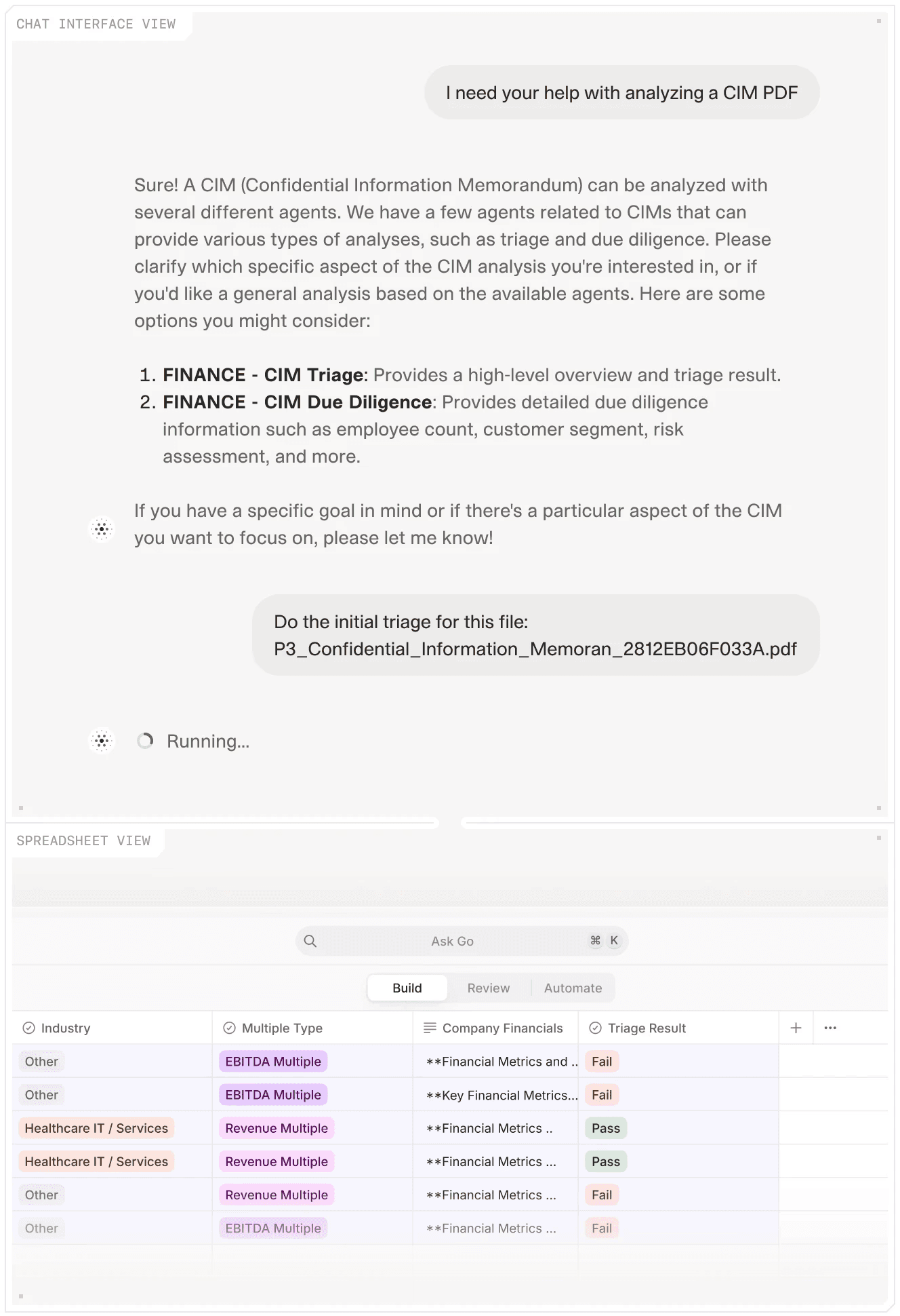
V7 Go runs CIM triage and due diligence agents in parallel, surfacing structured financial outputs alongside the original document for immediate analyst review.
The agent handles extraction, normalisation, and structuring. The analyst exercises judgment: are those add-backs legitimate? Is that exit multiple defensible given current conditions? What does the downside sensitivity look like if year-two revenue growth stalls?
The AI Financial Model Builder Agent extends this further: consolidated historical financials, a public comps table, and a structured data export ready to drop into the fund's house model. The same document inputs, formatted for the model rather than for human review.
For a team running five to twenty new deal CIMs a month, the difference in deal capacity is material. First-pass LBO analysis that previously took two days now takes under an hour. More deals reach a modelled first pass before any analyst time is committed. The ones that don't work get screened out faster.
What changes in the deal team's day-to-day is not the model but the conversation. When the first-pass analysis arrives before the team has finished reading the document, investment committee discussions can focus immediately on thesis questions rather than data questions. Is the FCF conversion assumption defensible? Is the exit multiple realistic given the current secondary buyer market? What's the downside case if the major customer churns? Those are the discussions that require a senior investor's judgment. Extracting EBITDA from page 78 of a CIM does not.
What the AI citation layer adds in a deal context
A common objection to AI-assisted financial analysis: extraction errors can compound through the model, and those errors are invisible until the deal has already moved forward.
V7 Go's AI Citations feature addresses this directly. Every figure extracted from the CIM, each revenue line, every EBITDA adjustment, any capex assumption, is linked back to the exact page and paragraph in the source document where it appears. Analysts reviewing the structured output can verify any input in seconds rather than re-reading the full document.
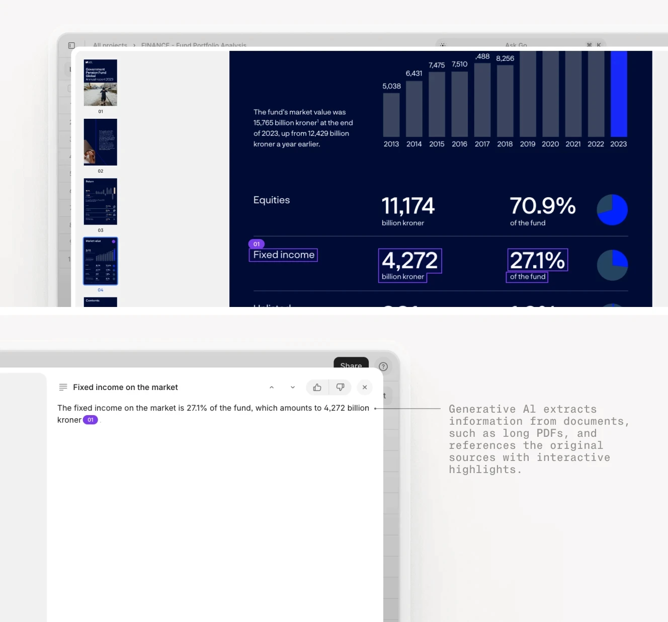
Every figure V7 Go extracts from a CIM is linked back to its exact source location in the original document, making verification a sampling exercise rather than a full re-read.
In a due diligence context, this traceability matters beyond efficiency. Investment committee documentation increasingly requires an audit trail showing how inputs were sourced and reviewed. A structured extraction log with page-level citations is that documentation, generated as a byproduct of the extraction itself.
The right LBO model doesn't guarantee a good outcome. What it does is tell you which assumptions the deal depends on, and whether those assumptions are realistic enough to bet on.
Deal teams using V7 Go across active PE pipelines describe the same shift: less time on document extraction before analysis can start, and more time on the decisions that actually require human judgment. The model is still built by the analyst. The first-pass financial inputs arrive before the analyst opens Excel.
The AI Investment Memo Generation automation extends this into downstream deal work: taking the structured output from the CIM analysis and producing a first-draft IC memo formatted to the fund's template. From CIM to modelled first pass to structured investment memo, without the three-day data sprint in the middle.
For a deal team running a meaningful volume of new opportunities each month, that changes what the pipeline looks like. More deals reach a modelled first pass before any team time is committed. The ones that don't work get screened out quickly. The ones that do get to the right questions sooner.

What is the difference between an LBO model and a DCF?
A DCF model is a valuation exercise: it projects future cash flows, applies a discount rate, and calculates an intrinsic value for the business independent of any transaction. An LBO model is a transaction exercise: it assumes an entry price, structures debt against it, projects cash flows over a hold period, and calculates the equity return at exit. The DCF asks what the company is worth. The LBO asks whether the deal works at this price. PE investors often run both on the same target: the DCF to check whether the entry multiple is defensible on a standalone valuation basis, the LBO to determine whether it meets the fund's return requirements. The key practical difference is orientation. The LBO starts from the required return and tests whether the entry price, debt structure, and operating assumptions are consistent with achieving it.
+
What is a good IRR for an LBO?
For middle-market buyout funds, target gross IRR typically falls in the range of 20 to 25%. This reflects the hurdle rate most institutional LPs expect PE funds to clear before the carried interest waterfall applies. Net IRRs, after management fees and carry, are typically 3 to 5 percentage points lower. In practice, the right IRR target is fund-specific and deal-specific. A lower-risk, contracted-revenue business at modest leverage might justify a 20% gross IRR target because the risk-adjusted return is attractive relative to public markets. A more cyclical, higher-leverage deal in a competitive sector might require 25 to 28% to justify the risk premium. Cambridge Associates tracks quarterly median and top-quartile PE returns by vintage year, which is the most reliable market reference for understanding where fund-level IRRs sit relative to peers.
+
What is MoIC in private equity?
MoIC stands for Multiple on Invested Capital. It is the total cash-on-cash return on equity invested in a transaction: if a fund invests $50M of equity and distributes $175M to LPs at exit, the MoIC is 3.5x. MoIC is time-agnostic and does not adjust for how long the capital was invested, which means it must be read alongside IRR for a complete picture of returns. A 3.5x MoIC over three years is a fundamentally different outcome from a 3.5x MoIC over eight years, even though the multiple is identical. In LP reporting, both metrics are shown together. DPI (Distributions to Paid-in Capital) is the realised equivalent of MoIC, the multiple based only on actual cash distributions to LPs, excluding any unrealised portfolio value still on the books.
+
What are the five components of an LBO model?
A standard LBO model is built from five structural blocks: entry assumptions and sources and uses, which define what is being paid and how it is funded at close; the debt schedule, which tracks how leveraged debt is repaid over the hold period from operating free cash flow; financial projections, which forecast revenue, EBITDA, capex, and working capital over three to seven years; exit assumptions, which estimate enterprise value at sale using projected EBITDA times an exit multiple; and the returns analysis, which calculates IRR and MoIC for the equity investor based on entry price, debt paydown, and exit proceeds. Most of the analytical complexity sits in the quality of the inputs to each block, particularly the normalised EBITDA figure at entry and the exit multiple assumption, rather than in the mechanics of the model structure itself.
+
What makes a company a good LBO candidate?
AI agents are being applied primarily to the data extraction and structuring work that precedes the LBO model, not to the model mechanics themselves. The most time-consuming part of deal analysis for most PE analysts is not building the model. It is extracting and normalising the financial inputs from a CIM: pulling historical revenue and EBITDA figures, tracking down add-back justifications, building a comparable transactions table, and structuring debt assumptions from current credit market data. AI agents trained on financial documents can read a CIM, extract and normalise these inputs, structure a sources and uses table, project a base case, and produce a first-pass LBO output with IRR and MoIC, with every figure cited back to its source page. This compresses two to three days of pre-model analyst work to under an hour. The investment judgment, whether the add-backs are defensible, whether the exit multiple assumption holds, whether the downside scenario is survivable, still belongs to the investor.
+
How is AI being used in LBO modeling?
Go is more accurate and robust than calling a model provider directly. By breaking down complex tasks into reasoning steps with Index Knowledge, Go enables LLMs to query your data more accurately than an out of the box API call. Combining this with conditional logic, which can route high sensitivity data to a human review, Go builds robustness into your AI powered workflows.
+
Casimir is a seasoned tech journalist and content creator specializing in AI implementation and new technologies. His expertise lies in LLM orchestration, chatbots, generative AI applications, and computer vision.

